import jax

jax.config.update("jax_enable_x64", True)  # use double-precision
jax.config.update("jax_persistent_cache_min_compile_time_secs", 0)
jax.config.update("jax_platforms", "cpu")
import jax.numpy as jnp
import matplotlib.pyplot as plt
from jax import Array
from tatva.plotting import (
    STYLE_PATH,
    colors,
)Appendix A — Basics of tatva
In this tutorial, we will get you started with the tatva package. The tatva is a tiny python package that provides a simple interface for performing finite element operations. We will use tatva to perform finite element operations, mainly:
- Interpolation of nodal values at quadrature points.
- Integration of functions over the domain.
- Gradients of nodal values at quadrature points.
Before we start, we need to import the essential packages i.e JAX, matplotlib and others for plotting.
To showcase how to perform all above mentioned operations using tatva, we define r a unit square domain with a triangular mesh. For ease, tatva provides a simple function Mesh.unit_square from tatva.Mesh module to generate square domain with a triangular mesh. The mesh object has the following attributes:
coords: The coordinates of the nodes in the mesh.elements: The elements in the mesh.
from tatva import Mesh

mesh = Mesh.rectangle((0, 1), (0, 1), 1, 1)
print("Coordinates of the nodes in the mesh: ", mesh.coords)
print("Connectivity of the elements in the mesh: ", mesh.elements)
Coordinates of the nodes in the mesh: [[0. 0.]
[0. 1.]
[1. 0.]
[1. 1.]]
Connectivity of the elements in the mesh: [[0 2 3]
[0 3 1]]Code: Plot the mesh.
plt.style.use(STYLE_PATH)
plt.figure(figsize=(2, 2), layout="constrained")
ax = plt.axes()
ax.tripcolor(
    *mesh.coords.T,
    mesh.elements,
    color="gray",
    lw=0.1,
    facecolors=jnp.ones(mesh.elements.shape[0]),
    cmap="managua_r",
)
ax.set_aspect("equal")
ax.set_xlabel("$x$")
ax.set_ylabel("$y$")
ax.margins(0.0, 0.0)
plt.show()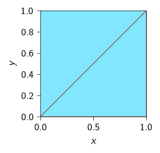
In order to perform finite element operations, we need to define an operator. To define an operator, we need to pass the mesh and the type of element used in that mesh to the tatva.Operator class. The Operator class takes the following arguments:
mesh: The mesh on which the operator is defined,tatva.Meshobject.element: The type of element used in the mesh,tatva.elementobject.
Since our mesh is a unit square domain with a triangular mesh, we can use the element.Tri3 class to define the type of element used in the mesh.
from tatva import Operator, element

tri = element.Tri3()
op = Operator(mesh, tri)
Evaluation at quadrature points
Tip
op.eval: Interpolate nodal values at quadrature points.
We can use the op to evaluate nodal values at the quadrature points. The function op.eval takes the nodal values and return the values at the quadrature points. The shape of the input array to the Operator.eval method is (n_nodes, n_dofs). And the shape of the output array is (n_elements, n_quadrature_points, n_dofs).
For example, below we evaluate the coordinate values of the mesh at the quadrature points. This basically means mapping the parameterized quadrature points (\(\in [-1, 1]^2\)) to the physical space.
quad_points_in_physical_space = op.eval(mesh.coords)

print(quad_points_in_physical_space.shape)
(2, 1, 2)In the above example, the shape of the output array is (2, 1, 2) because we have 2 elements in the mesh and 1 quadrature point in each element. And each element has 2 degrees of freedom (2 displacement components). To test whether the output is correct, we can plot the quadrature points in the physical space. Below, we plot the mesh and the quadrature points in the physical space.
Code: Plot the quadrature points in the physical space.
quad_points_in_physical_space = quad_points_in_physical_space.squeeze()

plt.style.use(STYLE_PATH)
plt.figure(figsize=(2, 2), layout="constrained")
ax = plt.axes()
ax.tripcolor(
    *mesh.coords.T,
    mesh.elements,
    color="gray",
    lw=0.1,
    facecolors=jnp.ones(mesh.elements.shape[0]),
    cmap="managua_r",
)
ax.scatter(
    quad_points_in_physical_space[:, 0],
    quad_points_in_physical_space[:, 1],
    c=colors.red,
    s=20,
    marker="x",
)
ax.set_aspect("equal")
ax.set_xlabel("$x$")
ax.set_ylabel("$y$")
ax.margins(0.0, 0.0)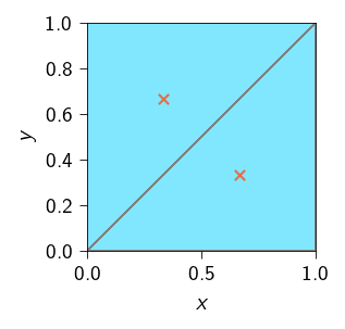
Gradients of nodal values
Tip
op.grad: Evaluate the gradient of nodal values at quadrature points.
As we discussed in Gradient of nodal values and strain tensor, we often need to evaluate the gradient of the nodal values at the quadrature points. For example, in the case of linear elasticity, we need to evaluate the gradient of the displacement field at the quadrature points to compute the strain tensor. The strain tensor is given as
\[ \boldsymbol{\epsilon}(x) = \dfrac{1}{2} \left( \nabla \boldsymbol{u}(x) + \nabla \boldsymbol{u}(x)^T \right) \]
where \(\nabla \boldsymbol{u}(x)=\left( \frac{\partial \boldsymbol{u}(x)}{\partial x_1}, \frac{\partial \boldsymbol{u}(x)}{\partial x_2}, \frac{\partial \boldsymbol{u}(x)}{\partial x_3} \right)\) is the gradient of the nodal displacements evaluated at point \(\boldsymbol{x}\).
The Operator class provides a method grad that can be used to evaluate the gradient of the nodal values at the quadrature points.
In this exercise, we will see how to use the Operator.grad method to evaluate the gradient of the nodal values at the quadrature points. For example, we want to compute the gradient of the coordinate values at the quadrature points.
\[ \nabla \boldsymbol{x} = \begin{bmatrix} \frac{\partial x}{\partial x} & \frac{\partial x}{\partial y} \\ \frac{\partial y}{\partial x} & \frac{\partial y}{\partial y} \end{bmatrix} \]
To do this, we can simply pass our nodal values (in this case, the coordinate values) to the Operator.grad function and it will return the gradient of the nodal values at the quadrature points. Remember to pass the nodal values to the Operator.grad function, it must be arranged in the shape (n_nodes, n_dofs).
op.grad(mesh.coords)Array([[[[1., 0.],
[0., 1.]]],
[[[1., 0.],
[0., 1.]]]], dtype=float64)As a sanity check, we can see that the gradient is an identity matrix since the gradient \(\partial x / \partial x = 1\) and \(\partial y / \partial y = 1\) and all other gradients are zero.
Important
The shape of the vector returned by the Operator.grad function is (n_elements, n_quadrature_points, n_dofs, n_dofs). The first dimension is the number of elements, the second dimension is the number of quadrature points, the third dimension is the number of degrees of freedom, and the fourth dimension is the number of degrees of freedom.
For a triangular element, the shape will be (n_elements, 1, 2, 2). For a quadrilateral element with 4 quadrature points, the shape will be (n_elements, 4, 2, 2).
The mathematical operation that Operator.grad performed internally are:
- Evaluate the nodal values at the quadrature points.
- Evaluate the gradient of the nodal values at the quadrature points using shape function matrix.
- Multiply the gradient of the nodal values with the Jacobian matrix.
- Return the gradient of the nodal values at the quadrature points.
Integrating a function over the domain
Tip
op.integrate: Integrate an array over the domain spanned by the operator’s mesh.
One basic operation that we require in FEM is to integrate a function over the domain. For example, integrating the strain energy density over the domain to get the total strain energy.
\[ \Psi_\text{e}(u) = \int_{\Omega} \frac{1}{2} \sigma : \epsilon \, dV \]
where \(\sigma\) is the stress tensor and \(\epsilon\) is the strain tensor evaluated at the quadrature points.
A finite element method way of integrating this over a discretized domain is to approximate the integral as a sum of integrals over the elements in the domain.
\[ \Psi_\text{e}(u) \approx \sum_{e \in \mathcal{E}} \sum_{\xi_1, \xi_2 \in \mathcal{Q}} \frac{1}{2} \sigma(\xi_1, \xi_2) : \epsilon(\xi_1, \xi_2) \, \text{det}\mathbf{J} \, w(\xi_1, \xi_2) \]
where \(\mathcal{E}\) is the set of all elements in the domain, \(\mathcal{Q}\) is the set of all quadrature points in the domain, \(J(\xi)\) is the Jacobian of the transformation from the reference element to the physical element, and \(\sigma(\xi)\) and \(\epsilon(\xi)\) are the stress and strain tensors evaluated at the quadrature point \(\xi\).
To do this, we can use the op.integrate method. The integrate method of the Operator class takes a function and returns the integral of the function over the domain.
For example, we want to integrate a function \(f(x, y)\) over the square domain we defined earlier i.e.
\[ \int_{\Omega} f(x, y) ~ dV = \sum_{e \in \mathcal{E}} \sum_{\xi_1, \xi_2 \in \mathcal{Q}} f(\xi_1, \xi_2) ~ \text{det}\mathbf{J} ~ w(\xi_1, \xi_2) \]
We will need the values of the function at the quadrature points \(f(\xi_1, \xi_2)\) and then pass it to the integrate method.
For this example, we assume that the function is constant and equal to 1.0. \[ f(x, y) = 1. \]
We will first define nodal values of the function. Since the function is constant, we can simply define the nodal values as an array of shape n_nodes.
f_nodal = jnp.full(mesh.coords.shape[0], fill_value=1.0)We can then evaluate the function at the quadrature points using the op.eval method.
f_at_quad = op.eval(f_nodal)And then can pass it to the integrate method.
op.integrate(f_at_quad)Array(1., dtype=float64)If you will notice the above integral is equal to 1 which also happens to be the area of the domain. This is not a coincidence. The integral of a constant function = 1 over a domain is the area of the domain. So this is a sanity check.
In the above example, we show how integrate method of the Operator class can be used to integrate a function over the domain. The function performs various operations under the hood such as:
- Looping over the elements in the mesh.
- Looping over the quadrature points in each element.
- Multiplying quadrature value with weights and determinant of the Jacobian matrix.
- Summing up the values over all the elements in the domain.
Tip
In the above example, we had a scalar value per node. But we may have vector values per node. For example, in the case of linear elasticity, we may have 2 displacement components per node. In that case, we can define the nodal values as an array of shape (n_nodes, 2). The above example can be extended to this case by evaluating the vector nodal values at the quadrature points and then passing it to the integrate method.
Interpolate a function over given points
Tip
op.interpolate: Interpolate nodal values at given points in the physical space.
Sometimes, we want to interpolate a function or nodal values over a given set of points. These set of points are in the physical space (not located at the nodes).
In this case, we need to first find the element that contains the point, then map the point to the reference space (in quadrature space) of that element. Once, we have the reference space coordinates, we can interpolate the function or nodal values at the quadrature points.
y_min = jnp.min(mesh.coords[:, 1])
y_max = jnp.max(mesh.coords[:, 1])
x_min = jnp.min(mesh.coords[:, 0])
x_max = jnp.max(mesh.coords[:, 1])
y = jnp.linspace(y_min, 0.9*y_max, 10)
x = jnp.full_like(y, fill_value=(x_min + x_max) / 2)

points = jnp.stack([x, y], axis=1)
op.interpolate(mesh.coords, points)Array([[0.5, 0. ],
[0.5, 0.1],
[0.5, 0.2],
[0.5, 0.3],
[0.5, 0.4],
[0.5, 0.5],
[0.5, 0.6],
[0.5, 0.7],
[0.5, 0.8],
[0.5, 0.9]], dtype=float64)