In this exercise, we will solve numerically the problem of contact between a elastic cylinder and a rigid plane. This is a classical problem in contact, called Hertz contact problem, for which we know the analytical solution. In this problem, a elastic cylinder is pressed against a rigid plane. The elastic cylinder is infinitely long and has a circular cross-section. Since the cylinder is infinitely long, we can consider a cross-section of the cylinder and solve a 2D problem. The schematic of the problem is shown below.
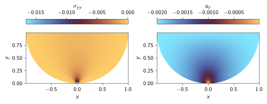
An animation of the elastic cylinder in contact with the rigid plane is shown below. The stress value shown is \(\sigma_{yy}\).
From Fundamentals, we know that the constraint condition for the contact between two bodies is given by:
where \(\boldsymbol{r}\) is the position vector of a point on the contact surface, \(\boldsymbol{\rho}\) is the position vector of the point on the target surface, and \(\boldsymbol{n}\) is the normal vector to the target surface.
For this problem, the target surface is the rigid plane and the contact surface is the surface of the elastic cylinder. The normal vector \(\boldsymbol{n}\) to the target surface is the \(+y\)-axis i.e.\(\boldsymbol{n} = (0, 1)\). Therefore, the constraint condition for the contact between the elastic cylinder and the rigid plane is given by:
\[
g_n = y - y_\text{rigid} \geq 0,
\]
where
\(y\) is the y-coordinate of a point on the contact surface of the elastic cylinder,
\(y_\text{rigid}\) is the y-coordinate of the rigid plane which is 0 for this problem.
The \(y-\)coordinate of the contact surface of the elastic cylinder is regularly updated as the elastic cylinder deforms. If the initial \(y-\)coordinate of the contact surface is \(y_0\), then the \(y-\)coordinate of the contact surface at any time \(t\) is given by \(y_0 + u_y\), where \(u_y\) is the \(y-\)displacement of the contact surface. Thus, the constraint condition for the contact between the elastic cylinder and the rigid plane is given by:
Since the rigid body is infinitely stiff, the deformable cylinder will deform so as to make contact with the rigid plane. The constraints are therefore on the displacements of the nodes of the contact surface of the deformable body. In this exercise, we will use the penalty method to enforce the constraints. The penalty method adds a penalty term to the objective function which penalizes the violation of the constraints. The objective function is given by:
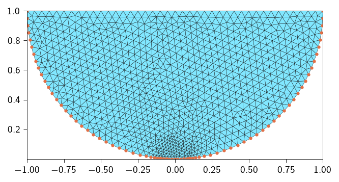
Below, we generate a triangular mesh of a half-circle. We also define a function to get the elements and nodes on the potential contact surface.
Function to generate a half-circle mesh and get the contact elements
import gmshimport meshiodef get_elements_on_curve(mesh, curve_func, tol=1e-3): coords = mesh.coords elements_2d = mesh.elements# Efficiently find all nodes on the curve using jax.vmap on_curve_mask = jax.vmap(lambda c: curve_func(c, tol))(coords) elements_1d = []# Iterate through all 2D elements to find edges on the curvefor tri in elements_2d:# Define the three edges of the triangle edges = [(tri[0], tri[1]), (tri[1], tri[2]), (tri[2], tri[0])]for n_a, n_b in edges:# If both nodes of an edge are on the curve, add it to the setif on_curve_mask[n_a] and on_curve_mask[n_b]:# Sort to store canonical representation, e.g., (1, 2) not (2, 1) elements_1d.append(tuple(sorted((n_a, n_b))))ifnot elements_1d:return jnp.array([], dtype=int)return jnp.array(elements_1d)def generate_half_circle_mesh( radius: float=1.0, mesh_size_fine: float=0.4, mesh_size_coarse: float=0.4, distance_from_rigid_plane: float=1e-3,):import os mesh_dir = os.path.join(os.getcwd(), "../meshes") os.makedirs(mesh_dir, exist_ok=True) output_filename = os.path.join(mesh_dir, "half_circle.msh")# Parameters R = radius # Radius of the half-circle gmsh.initialize() gmsh.model.add("half_circle")# Create points p1 = gmsh.model.geo.addPoint(0, R + distance_from_rigid_plane, 0) # Center p2 = gmsh.model.geo.addPoint(-R, R + distance_from_rigid_plane, 0) # Left point p3 = gmsh.model.geo.addPoint(R, R + distance_from_rigid_plane, 0) p4 = gmsh.model.geo.addPoint(0, distance_from_rigid_plane, 0) # Center# Create the arc (half-circle) arc = gmsh.model.geo.addCircleArc(p2, p1, p4) arc_2 = gmsh.model.geo.addCircleArc(p4, p1, p3)# Create the flat line to close the half-circle line = gmsh.model.geo.addLine(p3, p1) line_2 = gmsh.model.geo.addLine(p1, p2)# Create a line loop and surface loop = gmsh.model.geo.addCurveLoop([arc, arc_2, line, line_2]) surface = gmsh.model.geo.addPlaneSurface([loop])# Synchronize and mesh gmsh.model.geo.synchronize()# Create a Distance field to control mesh size near p_mid field_id = gmsh.model.mesh.field.add("Distance", 1) gmsh.model.mesh.field.setNumbers(field_id, "NodesList", [p4])# Create a Threshold field to refine near p_mid and coarsen further away thresh_field = gmsh.model.mesh.field.add("Threshold", 2) gmsh.model.mesh.field.setNumber(thresh_field, "InField", field_id) gmsh.model.mesh.field.setNumber(thresh_field, "SizeMin", mesh_size_fine) gmsh.model.mesh.field.setNumber(thresh_field, "SizeMax", mesh_size_coarse) gmsh.model.mesh.field.setNumber(thresh_field, "DistMin", R /8) gmsh.model.mesh.field.setNumber(thresh_field, "DistMax", R /4)# Set it as background mesh size field gmsh.model.mesh.field.setAsBackgroundMesh(thresh_field)# Generate the mesh gmsh.model.mesh.generate(2) gmsh.write(output_filename)print(f"Mesh successfully generated and saved to '{output_filename}'") gmsh.finalize() _mesh = meshio.read(output_filename) mesh = Mesh( coords=_mesh.points[:, :2], elements=_mesh.cells_dict["triangle"], ) contact_elements = get_elements_on_curve(mesh, contact_line, tol=1e-6)return mesh, contact_elements# get contact elements# function identifies nodes on the linedef contact_line(coord: jnp.ndarray, tol: float) ->bool:return jnp.isclose( jnp.linalg.norm(coord - jnp.array([0, radius + distance_from_rigid_plane])), radius, atol=1e-10, )
Below, we generate the mesh and get the contact elements. We assume the following parameters for the mesh:
radius of the half-circle: 1.0 \(\text{m}\)
initial distance from the rigid plane: 1e-6 \(\text{m}\)
fine mesh size along the expected contact region: 0.02, reducing this value will increase the number of elements along the contact region
coarse mesh size elsewhere: 0.05
Hint
The mesh plays a critical role in FEM solution. Since the contact is localized, we need to resolve the contact region properly. If the mesh is not fine enough, the solution will not give the correct results. You will see whether the above chosen value for the mesh size is fine enough as we proceed with the solution.
Let us define the material parameters mainly the shear modulus and the first Lamé parameter. The Youngs modulus and the Poisson’s ratio are related for the material are:
\[
E = 1.0 ~\text{N/m}^2, \quad \nu = 0.3
\]
From the above, we can compute the shear modulus and the first Lamé parameter as:
tri = element.Tri3()op = Operator(mesh, tri)@autovmap(grad_u=2)def compute_strain(grad_u: Array) -> Array:"""Compute the strain tensor from the gradient of the displacement."""return0.5* (grad_u + grad_u.T)@autovmap(eps=2)def compute_stress(eps: Array, mu: float, lmbda: float) -> Array:"""Compute the stress tensor from the strain tensor.""" I = jnp.eye(2)return2* mu * eps + lmbda * jnp.trace(eps) * I@autovmap(grad_u=2)def strain_energy(grad_u: Array, mu: float, lmbda: float) -> Array:"""Compute the strain energy density.""" eps = compute_strain(grad_u) sig = compute_stress(eps, mu, lmbda)return0.5* jnp.einsum("ij,ij->", sig, eps)@jax.jitdef total_strain_energy(u_flat: Array) ->float:"""Compute the total energy of the system.""" u = u_flat.reshape(-1, n_dofs_per_node) grad_u = op.grad(u) energy_density = strain_energy(grad_u, mat.mu, mat.lmbda)return op.integrate(energy_density)
Defining the contact energy
The contact energy is defined as:
\[
\Psi_\text{contact}(u)=\frac{1}{2}k_\text{pen}\int_{\Gamma_c}\Big\langle g_i(u)\Big\rangle^2 \text{d}\Gamma
\] where \(\Gamma_c\) is the contact surface, \(k_\text{pen}\) is the penalty parameter, and \(g(u)\) is the gap function.
For this exercise, we define the discrete penalization only at the nodes on the contact surface. Therefore, the contact energy is defined as:
where \(N_c\) is the number of nodes on the contact surface, \(a_i\) is the area of the node \(i\), and \(g_i(u)\) is the gap function at node \(i\).
Defining the penalty parameter
The penalty parameter \(k_\text{pen}\) is a parameter that controls the stiffness of the contact. It is a scalar parameter that is used to penalize the violation of the contact constraint.
Below define the penalty parameter \(k_\text{pen}\).
k_pen =1e6
Computing the area associated with each contact node
For correct resolution of the contact problem, we need the area associated with each contact node. In order to compute the area of each contact node, we define a line mesh that contains the contact nodes and the edges of the contact elements. We then define a function which integrates a constant field of value 1 over the line mesh.
where \(q(x)\) is a constant field of value 1. We can then compute the area of each node by differentiating the total area with respect to the field \(q(x)\).
In Figure 11.1, we consider all the potential contact nodes that can be in contact with the rigid plane highlighted in red. This will be our active set. In order to check which of these nodes violates the contact constraint \(g(u_i) \leq 0\), we will use the Macaulay’s bracket.
In the previous exercise, we used a Lagrange multiplier to enforce the contact constraint and therefore, we had set the \(\lambda_i\) to zero for the nodes which were not active. However, in the penalty method, we add \(k_\text{pen}\) to the stiffness matrix to enforce the contact constraint. Therefore, we need to make sure that where ever the contact constraint is violated, we do not add \(k_\text{pen}\) to the stiffness matrix at those locations.
By using the Macaulay’s bracket, we set the contact energy to zero for the nodes which are not in contact with the rigid plane.
In order to compute the contact energy, we need to compute the Macaulay’s bracket.
Below, define the functions to define the Macaulay’s bracket and then use that function to compute the contact energy.
Hint
The function for Macaulay’s bracket will look like this:
def macalauy_bracket(x: float) ->float:""" Computes the Macaulay bracket for the penalty method. This function should return x if x < 0, and 0 otherwise. """# TODO: Implement the Macaulay bracket using jnp.where(....)return ...§
To compute the contact energy, we will have to do the following:
Extract the displacements, coordinates, and areas for all the potential contact nodes.
Compute the gap function for each node.
Compute the penetration using the macaulay_bracket function you just wrote. This is applying the active set.
Compute the penalty energy for this single node: 0.5 _ k_pen _ penetration² * area.
Sum up all the individual nodal energies to get the total contact energy.
The function for the contact energy will look like this:
def compute_contact_energy( u: Array, coords: Array, contact_nodes: Array, nodes_area: Array) ->float:"""Compute the contact energy for a given displacement field. Args: u: Displacement field, shape (n_nodes, 2). coords: Initial coordinates of the nodes, shape (n_nodes, 2). contact_nodes: Indices of all the nodes on the contact surface, shape (n_contact_nodes,). nodes_area: Area of all the nodes in the mesh, shape (n_nodes,). Returns: Contact energy, a scalar. """# TODO Extract the displacements, coordinates, and areas for ONLY the contact_nodes. u_nodes = ... x_nodes = ... contact_nodes_area = ...# TODO Define a helper function that calculates the energy for a SINGLE node.# This function will be vectorized in the next step.def contact_energy_node(u_node: tuple[float, float], x_node: tuple[float, float], contact_area : float) ->float:""" Computes the contact energy for a single node Args: u_node: displacements for a node (u_x, u_y) x_node: initial coordinate of a node (x, y) contact_area: area associated with a node """# Calculate the gap 'g_n'. gap = ...# Calculate the penetration using the macaulay_bracket function you just wrote. penetration = ...# Compute the penalty energy for this single node: 0.5 * k_pen * penetration² * area.return ...# TODO Vectorize the single-node function using jax.vmap.# This creates a new function that can process all nodes at once.# The in_axes argument should be (0, 0, 0) because we are iterating over the# first axis of u_nodes, x_nodes, and area_nodes. contact_energy_vmap = jax.vmap(...)# TODO Call the vectorized function with the arrays of nodal data you extracted in Step 1. all_nodal_energies = contact_energy_vmap(...)# TODO Sum up all the individual nodal energies to get the total contact energy.return ...
@jax.jitdef macaulay_bracket(x):return jnp.where(x >0, 0, x)@jax.jitdef compute_contact_energy( u: Array, coords: Array, contact_nodes: Array, nodes_area: Array) -> Array:"""Compute the contact energy for a given displacement field. Args: u: Displacement field. coords: Coordinates of the nodes. contact_nodes: Indices of the nodes on the contact surface. nodes_area: Area of the nodes on the contact surface. Returns: Contact energy. """ u_nodes = u[contact_nodes] x_nodes = coords[contact_nodes] contact_nodes_area = nodes_area[contact_nodes]# Loop over nodes on the potential contact surfacedef _contact_energy_node( u_node: tuple[float, float], x_node: tuple[float, float], contact_area: float ) ->float: gap = (x_node[1] + u_node[1]) -0.0 penetration = macaulay_bracket(gap)return0.5* k_pen * (penetration**2) * contact_area contact_energy_node = jax.vmap(_contact_energy_node, in_axes=(0, 0, 0))return jnp.sum(contact_energy_node(u_nodes, x_nodes, contact_nodes_area))
def total_energy( u_flat: Array, coords: Array, contact_nodes: Array, nodes_area: Array,) ->float:"""Compute the total energy for a given displacement field. Args: u_flat: Flattened displacement field, shape (n_dofs,). coords: Initial coordinates of the nodes, shape (n_nodes, 2). contact_nodes: Indices of the nodes on the contact surface, shape (n_contact_nodes,). nodes_area: Area of the nodes on the contact surface, shape (n_nodes,). Returns: Total energy, a scalar """# TODO compute the contact energy contact_energy = ...# TODO compute the elastic energy strain_energy = ...# TODO Sum the contact and strain energies to get the total energy of the system.return ...
@jax.jitdef _total_energy( u_flat: Array, coords: Array, contact_nodes: Array, nodes_area: Array,) -> Array:"""Compute the total energy for a given displacement field. Args: u_flat: Flattened displacement field. coords: Coordinates of the nodes. contact_nodes: Indices of the nodes on the contact surface. nodes_area: Area associated with all the nodes in the mesh Returns: Total energy. """ u = u_flat.reshape(-1, n_dofs_per_node) contact_energy = compute_contact_energy( u, coords, contact_nodes, nodes_area ) strain_energy = total_strain_energy(u)return contact_energy + strain_energytotal_energy = partial( _total_energy, coords=mesh.coords, contact_nodes=contact_nodes, nodes_area=nodes_area,)
Computing the internal forces and the stiffness matrix
For this exercise, we will like to use the sparse solver, given the large number of degrees of freedom. We will use the sparse module to compute the sparsity pattern and then use the sparse.jacfwd to compute the Jacobian of the internal forces.
We make use of the sparse.create_sparsity_pattern to define the sparsity pattern of the problem. Below, we define steps to:
Create the sparsity pattern
Compute the internal force vector from the total energy using jax.jacrev
Compute the sparse stiffness matrix from the internal force vector using sparse.jacfwd and the sparsity pattern
Hint
Be careful when defining the sparsity pattern. Unlike the previous exercises, where we had extra degrees of freedom for lagrange multipliers, here we have only the displacement degrees of freedom. So the sparsity pattern would only be dependent on the mesh and the number of displacement dofs per node.
We push the deformable cylinder into the rigid plane by applying a displacement in the \(y\) direction on the top edge of the cylinder. To avoid rigid body motion, we fix the displacement in the \(x\) direction on the top edge of the cylinder. The boundary conditions thus applied are:
\[
\begin{aligned}
u_y &= -R/500 \quad \text{on the top edge} \\
\end{aligned}
\]
where \(R\) is the radius of the cylinder.
Hint
Get the nodes on the top edge of the cylinder and then get the dofs associated with those nodes.
top_nodes =# get unique nodes from the interface_elementsfixed_dofs = [dofs_associated_with_top_nodes_in_y_direction]
We apply boundary conditions using the lifting approach. To apply the lifting to a sparse stiffness matrix, we need the indices corresponding the rows and columns that are fixed (to be set to zero) and the indices of the diagonal elements that are set to one.
Below use the sparse.get_bc_indices to get the indices (row, col) where we set the stiffness entries to zero and the indices of the diagonal elements that are set to one.
We will use the Newton’s method to solve the problem. Remember we use the lifting approach to apply the boundary conditions, therefore, we need to modify the stiffness matrix and the residual vector to account for the boundary conditions. See Sparse solvers for more details on how to use the lifting approach within a Newton solver.
Hint
The Newton solver will look like this:
import scipy.sparse as spfrom jax import Arrayimport jax.numpy as jnpdef newton_sparse_solver( u: Array, fext: Array, gradient: callable, hessian_sparse: callable, fixed_dofs: Array, zero_indices: Array, one_indices: Array, ..., ...) ->tuple[Array, float]:"""Solves the nonlinear system using Newton's method with a sparse direct solver. Args: u: Current displacement field, shape (n_dofs,). fext: External force vector, shape (n_dofs,). gradient: Function to compute the internal forces hessian_sparse: Function to compute the sparse stiffness matrix fixed_dofs: Indices of the fixed degrees of freedom where we apply the Dirichlet boundary conditions, shape (n_fixed_dofs,). zero_indices: Indices of the rows and columns to set to zero in the stiffness matrix, because of the Dirichlet boundary conditions, one_indices: Indices of the diagonal elements to set to one in the stiffness matrix, because of the Dirichlet boundary conditions. ...: Any other arguments required by the gradient and hessian_sparse functions. ...: Any other arguments required by the gradient and hessian_sparse functions. Returns: u: Displacement field, shape (n_dofs,). norm_res: Norm of the residual, a scalar. """ fint = gradient(u) iiter =0 norm_res =1.0 tol =1e-8 max_iter =10while norm_res > tol and iiter < max_iter:# TODO: Calculate the residual vector R = F_ext - F_int.# For the lifting method, the residual at the fixed DOFs must be set to zero. residual = ...# TODO: Compute the sparse stiffness matrix K at the current displacement u. K_sparse = ...# TODO: Apply the lifting method to modify the stiffness matrix data.# "Zero out" the rows/columns for the fixed DOFs and set the diagonal to 1.# Use the indices for these operations (zero_indices, one_indices) K_data_lifted = ...# TODO: Reconstruct the modified scipy.sparse.csr_matrix for the solver.# Use the modified data `K_data_lifted` and the original indices from `K_sparse`. K_csr = ...# TODO: Solve the modified linear system K_mod * du = R_mod for the update `du`.# Use the direct solver: scipy.sparse.linalg.spsolve. du = ...# TODO: Update the total displacement vector u. u = ...# TODO: Re-compute the internal forces `fint` at the new position `u`# to get the latest residual for the convergence check. fint = ...# TODO: Calculate the new residual and its norm.# Again, remember to zero out the residual at the fixed DOFs before taking the norm. residual = ... norm_res = ...print(f" Residual: {norm_res:.2e}") iiter +=1return u, norm_res
Now that we have the mesh, the energy functions, and the newton_sparse_solver, it’s time to set up the main simulation loop. We will apply the displacement in small increments and solve for equilibrium at each step. This is important because using penalty method, the problem becomes non-linear and the solution is sensitive to the initial guess.
Follow these steps to build the main part of your script.
Hint
Initialization
Before the loop, you need to initialize all the variables for the simulation.
Create the initial solution vector u_prev, which contains both displacements. Initialize it as a vector of zeros with the correct total size (n_dofs).
Initialize the external force vector fext as a vector of zeros.
Set the number of load increments, n_steps (e.g., 10). We would apply the total applied_displacement in n_steps.`
Calculate the displacement to apply at each step.
The Main Loading Loop
Create a for loop that iterates through each load step.
for step inrange(n_steps):print(f"Step {step+1}/{n_steps}")# ... Your code for each step will go inside this loop ...
Inside the Loop: Apply Displacement and Prepare Solver
At the beginning of each loop iteration, you need to update the boundary conditions and prepare the functions for the solver.
Update the u_prev vector with the prescribed displacement for the current step.
Inside the Loop: Solve for Equilibrium
Call the newton_sparse_solver function with the initial guess and other arguments. Depending on what inputs your gradient and hessian_sparse functions require, you may need to pass additional arguments to the newton_sparse_solver function. You will also have to pass the fixed_dofs, zero_indices, and one_indices to the newton_sparse_solver function to apply the lifting method.
Store the new solution in u_new.
Update the state for the next iteration by setting u_prev = u_new. This is basically providing the solution from the previous step as the initial guess for the next step., which helps the solver converge faster.
After the Loop: Final Solution
Once the loop is complete, extract the final displacement field from the final u_prev vector for visualization.
Figure 11.2: Stress field \(\sigma_{yy}\) after the contact is resolved. The undeformed configuration is shown in the background.
Checking the effect of penalty parameter on the gap function
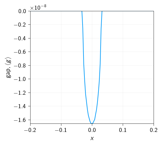
Since, we used the penalty approach, the nodes are not exactly on the contact surface but depending on the penalty parameter, they will penetrate the surface. Let us see how the gap function looks like at the contact surface.
Code: Plot the zoomed in contact surface to see the node locations.
Figure 11.3: Zoomed in contact surface to see the node locations. We see that there is some interpenetration due to the penalty parameter.
The above results looks good but we do not know whether the solution that we get is correct. We do have convergence at each applied displacement but we do not know whether the solution is correct.
Therefore, to verify the solution, we can compare the solution with Hertz theory that is explained in Fundamentals.
Comparing numerical results with Hertz contact theory
As mentioned earlier, the Hertz solution is characterized by a contact radius \(a\) and a contact pressure \(p_0\). The contact radius \(a\) is given by,
where \(P\) is the load and \(E^{\star}\) is the effective Young’s modulus of the cylinder. For plain strain condition, the effective Young’s modulus is given by, \[
E^* = \frac{E}{1-\nu^2}
\]
Below compute the contact radius \(a\) and the contact pressure \(p_0\) from Hertz theory.
P = f_contactE_eff = E / (1- nu**2) # effective Young's modulus for plain strain conditiona0 = np.sqrt(4* P * radius / jnp.pi / E_eff)p0 =2* P / jnp.pi / a0x_hertz = np.linspace(-a0, a0, 100)x_hertz = x_hertz[x_hertz !=0]p_hertz =2* P * np.sqrt(a0**2- x_hertz**2) / jnp.pi / a0**2print(f"Contact radius from Hertz theory {a0}")print(f"Contact pressure from Hertz theory {p0}")
Contact radius from Hertz theory 0.03022952413571173
Contact pressure from Hertz theory 0.016609628645995456
Comparing contact pressure profile with Hertz theory
Based on Hertz theory, the traction profile along the contact surface is given by,
\[
p(r) = -p_0 \sqrt{1-(\frac{r}{a})^2}
\]
where \(r\) is the radial distance from the center of the contact surface and it varies from \(-a\) to \(a\).
Now, we will extract the surface tractions \(t_n = \boldsymbol{\sigma} : \boldsymbol{n}\) along the contact surface from our numerical solution, where \(\boldsymbol{n}\) is the normal vector to the contact surface and \(\boldsymbol{\sigma}\) is the stress tensor in the elements along the contact surface. Below we have defined a function to extract the surface tractions from the numerical solution. This function calculates the surface traction \(t_n\) along the contact surface for each element and returns the points, tractions, and normals of the surface elements.
Use this function to extract the surface tractions.
Code: Function to extract surface tractions
def get_surface_tractions( surface_elements: np.ndarray, mesh: Mesh, element_values: jnp.ndarray,) -> np.ndarray:""" Finds triangle elements that share a common edge with given surface elements, For each triangle element, it computes the traction on the surface element. It returns the points, tractions, and normals of the surface elements. Args: surface_elements (np.ndarray): An array of surface connectivity, shape (num_surface_elements, 2). mesh (Mesh): A mesh object. element_values (jnp.ndarray): An array of element values, shape (num_elements,). Returns: np.ndarray: An array of points, shape (num_surface_elements, 2). np.ndarray: An array of tractions, shape (num_surface_elements, 2). np.ndarray: An array of normals, shape (num_surface_elements, 2). """ line_edge_set = {tuple(sorted(edge)) for edge in surface_elements} tractions = [] points = [] normals = []for i, tri inenumerate(mesh.elements): p1, p2, p3 = tri edges = [tuple(sorted((p1, p2))),tuple(sorted((p2, p3))),tuple(sorted((p3, p1))), ]for edge in edges:if edge in line_edge_set: stress_value = element_values[i] coords = np.array([mesh.coords[edge[0]], mesh.coords[edge[1]]]) tangent_vector = coords[1] - coords[0] normal = jnp.array([-tangent_vector[1], tangent_vector[0]]) normal = normal / jnp.linalg.norm(normal) traction = stress_value @ normal mid_point = jnp.mean(coords, axis=0) tractions.append(traction) points.append(mid_point) normals.append(normal)breakreturn np.array(points), np.array(tractions)
Below we call the function get_surface_tractions to extract the surface tractions. The surface tractions are stored in the variable surface_tractions and the surface points are stored in the variable surface_points.
Once you have the surface tractions, you should plot the traction profile along the contact surface. Also plot the \(p(r)\) from Hertz theory and see if they match.
Plot the numerical Contact Pressure (from your simulation):
X-axis: The x-coordinates of the nodes on the contact surface (surface_points).
Y-axis: The magnitude of the contact pressure from your simulation. This is the absolute value of the y-component of the surface_tractions.
Plot the Analytical Hertzian Pressure:
X-axis: The array of x-coordinates from the Hertzian calculation, you can either use the surface_points or define a new array of x-coordinates for smoother curve.
Y-axis: The array of corresponding pressure values from the Hertzian calculation.
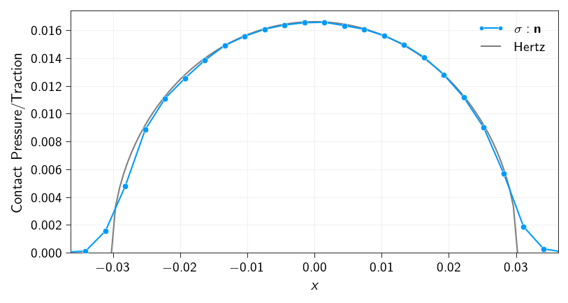
Figure 11.4: Profile of traction normal (\(t_n = \boldsymbol{\sigma} : \boldsymbol{n}\)) to the curved surface computed from the numerical solution (blue) and compare it with Hertz theory (gray).
Does the numerical solution match with Hertz theory?
Do you think the numerical solution matches with Hertz theory? Why or why not?
If doesnot match, what is the reason for the mismatch? Is it due to the penalty parameter? Is it due to the fact the mesh is not fine enough at the contact surface?
Try to improve the match by changing the penalty parameter and the mesh.
Comparing stresses inside of the cylinder with Hertz theory
We also compare the stresses inside of the cylinder along the line \(x=0\) with Hertz theory. According to Hertz theory, the stresses are given by:
Below define a function to compute the stresses inside of a body based on Hertz solution.
Hint
The function definition will be something like this:
def hertz_solution(x, y, a0, p0):"""Compute the stresses based on Hertz solution. Args: x (float): The x-coordinate of the point. y (float): The y-coordinate of the point. a0 (float): The contact radius. p0 (float): The contact pressure. Returns: tuple: A tuple of three floats representing the $\sigma_{xx}$, $\sigma_{yy}$, and $\sigma_{xy}$ stresses. """# TODO:Compute the stresses based on Hertz solution ...# Return the stressesreturn sigma_x, sigma_y, sigma_xy
Code: Function to compute the stresses based on Hertz solution
Code: Function to find the index of the containing polygon for each point.
import numpy as np@jax.jitdef find_containing_polygons( points: jnp.ndarray, polygons: jnp.ndarray,) -> jnp.ndarray:""" Finds the index of the containing polygon for each point. This function uses a vectorized Ray Casting algorithm and is JIT-compiled for maximum performance. It assumes polygons are non-overlapping. Args: points (jnp.ndarray): An array of points to test, shape (num_points, 2). polygons (jnp.ndarray): A 3D array of polygons, where each polygon is a list of vertices. Shape (num_polygons, num_vertices, 2). Returns: jnp.ndarray: An array of shape (num_points,) where each element is the index of the polygon containing the corresponding point. Returns -1 if a point is not in any polygon. """# --- Core function for a single point and a single polygon ---def is_inside(point, vertices): px, py = point# Get all edges of the polygon by pairing vertices with the next one p1s = vertices p2s = jnp.roll(vertices, -1, axis=0) # Get p_{i+1} for each p_i# Conditions for a valid intersection of the horizontal ray from the point# 1. The point's y-coord must be between the edge's y-endpoints y_cond = (p1s[:, 1] <= py) & (p2s[:, 1] > py) | (p2s[:, 1] <= py) & ( p1s[:, 1] > py )# 2. The point's x-coord must be to the left of the edge's x-intersection# Calculate the x-intersection of the ray with the edge x_intersect = (p2s[:, 0] - p1s[:, 0]) * (py - p1s[:, 1]) / ( p2s[:, 1] - p1s[:, 1] ) + p1s[:, 0] x_cond = px < x_intersect# An intersection occurs if both conditions are met. intersections = jnp.sum(y_cond & x_cond)# The point is inside if the number of intersections is odd.return intersections %2==1# --- Vectorize and apply the function ---# Create a boolean matrix: matrix[i, j] is True if point i is in polygon j# Vmap over points (axis 0) and polygons (axis 0)# in_axes=(0, None) -> maps over points, polygon is fixed# in_axes=(None, 0) -> maps over polygons, point is fixed# We vmap the second case over all points is_inside_matrix = jax.vmap(lambda p: jax.vmap(lambda poly: is_inside(p, poly))(polygons) )(points)# Find the index of the first 'True' value for each point (row).# This gives the index of the containing polygon.# We add a 'False' column to handle points outside all polygons.# jnp.argmax will then return the index of this last column. padded_matrix = jnp.pad( is_inside_matrix, ((0, 0), (0, 1)), "constant", constant_values=False ) indices = jnp.argmax(padded_matrix, axis=1)# If the index is the last one, it means the point was not in any polygon.# We map this index to -1 for clarity.return jnp.where(indices == is_inside_matrix.shape[1], -1, indices)
Next, we will compute the stresses along the line \(x=0\) from our numerical solution and compare them with the stresses from Hertz theory.
Below, we define a set of points along the line \(x=0\) and find the element indices of the containing polygons for each point. We use the function find_containing_polygons to find the element indices. Then we select the stresses from the stress tensor for the corresponding element indices.
The stresses are stored in the variable stresses_along_points which is a 3D array of shape \((n, 2, 2)\) where \(n\) is the number of points. The first dimension corresponds to the points, the second dimension corresponds to the stress components, and the third dimension corresponds to the stress tensor. We will plot different components of the stress tensor along the line \(x=0\) and compare them with solution from Hertz theory as discussed above.
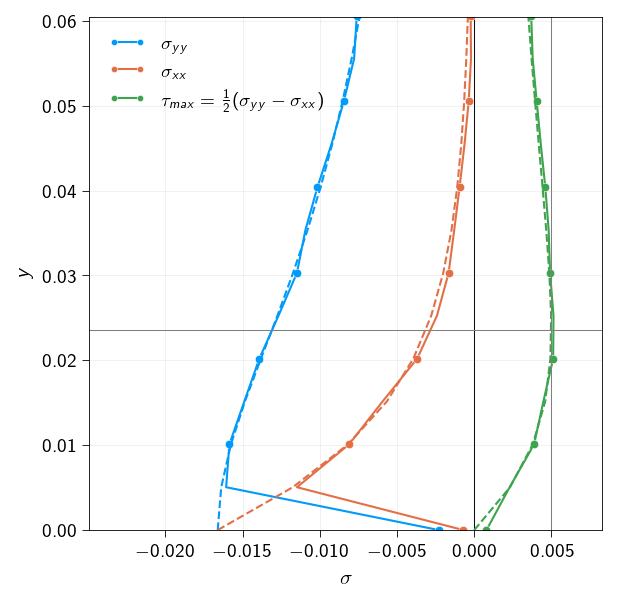
Below, we plot the stresses (\(\sigma_{yy}, \sigma_{xx}, \tau_{max}\)) along the line \(x=0\) from the numerical solution and compare them with the stresses from Hertz theory.
In the plot, plot the stresses along the \(x-\) axis and the \(y-\) coordinates along the \(y-\) axis.
Figure 11.5: Stresses along the line \(x=0\) from the numerical solution (in solid line) and comparison with Hertz theory (in dashed line)
Does the numerical solution match with Hertz theory?
Do you think the numerical solution matches with Hertz theory? Why or why not? Try to improve the match by changing the penalty parameter and the mesh.