Dirichlet BC as constraints (Penalty method)

In this exercise, we will see an application of constraint handling in FEM and we will apply Dirichlet boundary conditions as constraints. The problem is the same as in the previous exercises.

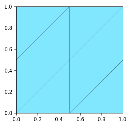
We have a unit square domain \(\Omega = [0, 1] \times [0, 1]\) which fixed in space in both \(x\) and \(y\) directions on the left edge. We apply a displacement along \(x-\)direction on the right edge. The applied displacement is \(0.3\). Furthermore, the domain is discretized using triangular elements.

The assumptions that we make in this exercise are:

linear elastic material
infinitesimal strains under plain strain conditions

In this exercise, we explore the constrained problem with:

equality constraint i.e \(g_i(u) = 0\)
active set is known and does not change i.e we always know which degrees of freedom are in \(\mathcal{A}\)

Thus, our constrained problem is

\[ \min_{\boldsymbol{u}} \Psi(\boldsymbol{u}) \]

\[ \text{such that} \quad g_i(u) = 0 \quad \forall i \in \mathcal{A} \]

Objective

The objective of this exercise is to use the penalty method to enforce the Dirichlet boundary conditions. We will use the penalty method to enforce the Dirichlet boundary conditions on the right edge as well as the left edge of the domain. Later, we will see how the value of the penalty parameter \(k_\text{pen}\) affects the solution.

Below is the expected workflow for solving this exercise.

Workflow

As we have mentioned, our way of solving any problem in this course is to define a python function that computes the total potential energy \(\Psi\).

For this specific problem, the total potential energy \(\Psi\) is given as

\[ \Psi(u) = \Psi_\text{e}(u) + \Psi_\text{pen}(u) - \boldsymbol{f}_\text{ext} \cdot \boldsymbol{u} \]

where

\(\Psi_\text{e}\) is the elastic strain energy
\(\Psi_\text{pen}\) is the penalty energy due to the Dirichlet boundary conditions
\(\boldsymbol{f}_\text{ext}\) is the external force vector which is zero in this case

Our task is to define the functions to compute the elastic strain energy, the penalty energy and the total potential energy.

Code: Importing the essential libraries

import jax

jax.config.update("jax_enable_x64", True)  # use double-precision
jax.config.update("jax_persistent_cache_min_compile_time_secs", 0)
jax.config.update("jax_platforms", "cpu")
import jax.numpy as jnp
from jax import Array

from tatva import Mesh, Operator, element, sparse
from tatva.plotting import STYLE_PATH, plot_element_values, plot_nodal_values
from jax_autovmap import autovmap

from typing import NamedTuple

from functools import partial

import numpy as np

import matplotlib.pyplot as plt

Model setup

Similar to previous exercises, we consider a unit square domain \(\Omega = [0, 1] \times [0, 1]\) which fixed in space in both \(x\) and \(y\) directions on the right edge. We apply a displacement along \(x-\)direction on the left edge. Furthermore, the domain is discretized using triangular elements.

mesh = Mesh.unit_square(2, 2)

n_nodes = mesh.coords.shape[0]
n_dofs_per_node = 2
n_dofs = n_dofs_per_node * n_nodes

Code: Plot unit square mesh

plt.style.use(STYLE_PATH)
plt.figure(figsize=(3, 3))
plt.tripcolor(
    *mesh.coords.T,
    mesh.elements,
    facecolors=jnp.ones(mesh.elements.shape[0]),
    edgecolors="k",
    lw=0.2,
    cmap="managua_r",
)
plt.gca().set_aspect("equal")
plt.gca().margins(0, 0)
plt.show()

Defining material parameters

Let us define the material parameters mainly the shear modulus and the first Lamé parameter.

\[ \mu = 0.5, \quad \lambda = 1.0 \]

class Material(NamedTuple):
    """Material properties for the elasticity operator."""

    mu: float  # Shear modulus
    lmbda: float  # First Lamé parameter


mat = Material(mu=0.5, lmbda=1.0)

Defining the total elastic energy

We would now define a function that computes the total energy of the system.

\[ \Psi_\text{e}(\boldsymbol{u}) = \int_\Omega \psi_\text{e}(\boldsymbol{\varepsilon}) d\Omega \]

where

\[ \psi_\text{e}(x) = \frac{1}{2} \boldsymbol{\sigma}(x) : \boldsymbol{\varepsilon}(x) \]

where \(\boldsymbol{\sigma}\) is the stress tensor and \(\boldsymbol{\varepsilon}\) is the strain tensor.

\[ \boldsymbol{\sigma} = \lambda \text{tr}(\boldsymbol{\varepsilon}) \mathbf{I} + 2\mu \boldsymbol{\varepsilon} \]

and

\[ \boldsymbol{\varepsilon} = \frac{1}{2} (\nabla \boldsymbol{u} + \nabla \boldsymbol{u}^T) \]

Hint

To do so, we must perform the following steps:

Define the triangular element from tatva.element.
Define the Operator object from tatva.operator which takes the mesh and the element as input.
Define the function that computes the total energy by performing following operations:
- Compute the gradient of the displacement, uses Operator.grad.
- Compute the strain energy density, use the function defined above
- Integrate the strain energy density over the domain, use Operator.integrate.

Code: Defining the material properties and the strain energy density

tri = element.Tri3()
op = Operator(mesh, tri)


@autovmap(grad_u=2)
def compute_strain(grad_u: Array) -> Array:
    """Compute the strain tensor from the gradient of the displacement."""
    return 0.5 * (grad_u + grad_u.T)


@autovmap(eps=2, mu=0, lmbda=0)
def compute_stress(eps: Array, mu: float, lmbda: float) -> Array:
    """Compute the stress tensor from the strain tensor."""
    I = jnp.eye(2)
    return 2 * mu * eps + lmbda * jnp.trace(eps) * I


@autovmap(grad_u=2, mu=0, lmbda=0)
def strain_energy(grad_u: Array, mu: float, lmbda: float) -> Array:
    """Compute the strain energy density."""
    eps = compute_strain(grad_u)
    sig = compute_stress(eps, mat.mu, mat.lmbda)
    return 0.5 * jnp.einsum("ij,ij->", sig, eps)


@jax.jit
def total_elastic_energy(u_flat: Array) -> float:
    """Compute the total energy of the system."""
    u = u_flat.reshape(-1, n_dofs_per_node)
    u_grad = op.grad(u)
    energy_density = strain_energy(u_grad, mat.mu, mat.lmbda)
    return op.integrate(energy_density)

Defining Dirichlet boundary conditions as constraints

We now define the degrees of freedom that for the left edge of the domain and the right edge of the domain. These are the degrees of freedom that are associated with the nodes on the left and right edge of the domain.

Remember that on the left edge, we have both \(x\) and \(y\) degrees of freedom fixed (\(u_x=u_y=0\)) and on the right edge, we have apply a displacement of 0.3 on \(x\) degree of freedom (\(u_x=0.3\)).

Hint

It might be best to store all the degrees of freedom where displacement is applied (either 0 or 0.3) as vector named constrained_dofs.

constrained_dofs = [dofs_associated_with_left_nodes, dofs_associated_with_right_nodes]

Also, we define total number of constraints nb_cons as

nb_cons = len(constrained_dofs)

left_nodes = jnp.where(jnp.isclose(mesh.coords[:, 0], 0.0))[0]
right_nodes = jnp.where(jnp.isclose(mesh.coords[:, 0], 1.0))[0]
constrained_dofs = jnp.concatenate(
    [
        2 * left_nodes,
        2 * left_nodes + 1,
        2 * right_nodes,
    ]
)

free_dofs = jnp.setdiff1d(jnp.arange(n_dofs), constrained_dofs)


applied_displacement = 0.3

prescribed_values = jnp.zeros(n_dofs).at[2 * right_nodes].set(applied_displacement)

We now define a constraints that enforces the Dirichlet boundary conditions on the degrees of freedom associated with the nodes on the right edge of the domain. Let us denote the applied displacement as \(u_d\). The constraint then is defined as

\[ u_x^{i} = u_d \quad \forall i \in \mathcal{A} \]

where \(\mathcal{A}\) is the set of degrees of freedom associated with the nodes on the right edge and the left edge of the domain.

We can define the constraint as a function of the degrees of freedom as follows:

\[ g_i(u) = u_{x}^{i} - u_d \]

Below define a function that computes the equality constraints as defined above.

Hint

The function should take the displacement vector \(u\) and the constraints as input and return the difference between the displacement vector and the constraints. The difference should be computed only for the degrees of freedom that are associated with the nodes on the left and right edge of the domain.

The function definition will be something like this:

def equality_constraints(u, constraints):
    """Compute the constraint vector g(u)
    
    Args:
        u: the displacement vector, a vector of size (n_dofs + nb_cons)
        constraints: the applied displacement at the constrained_dofs, a vector of size (nb_cons)
    
    Returns:
        the constraint vector, a vector of size (nb_cons)
    """

    # get the displacement values at constrained_dofs from u
    ...
    # compute the g(u) i.e. difference between the above displacement values and the applied displacement
    ...
    # return the constraint vector
    return ...

nb_cons = len(constrained_dofs)

@jax.jit
def equality_constraints(u, constraints):
    return u.at[constrained_dofs].get() - constraints

Defining the total potential energy

The total potential energy \(\Psi\) is the sum of the elastic strain energy \(\Psi_\text{e}\) and the contact penalty energy \(\Psi_\text{pen}\).

\[\Psi(u)=\Psi_\text{e}(u)+\Psi_\text{pen}(u) - \boldsymbol{f}_\text{ext} \cdot \boldsymbol{u}\]

where \(\Psi_\text{e}\) is the elastic strain energy and \(\Psi_\text{pen}\) is the penalty energy. We have already defined \(\Psi_\text{e}\) in the previous section. We now define \(\Psi_\text{pen}\) as

\[ \Psi_\text{pen}(u) = \frac{k_\text{pen}}{2} \sum_{i \in \mathcal{A}} \left( g_i(u) \right)^2 \]

where \(k_\text{pen}\) is the penalty parameter.

For starting we choose a small value of \(k_\text{pen}=10^{-1}\) to see if the constraints are satisfied.

Later, we will modify this value to see the effect of the penalty parameter on the solution.

k_pen = 1e-1

Write a function that computes the penalty energy term as defined above (using the k_pen) and the total potential energy as defined above.

Hint

The function definition will be something like this:

def penalty_energy(u, constraints):
    """Compute the penalty energy term

    Args:
        u: the displacement vector, a vector of size (n_dofs)
        constraints: the applied displacement at the constrained_dofs, a vector of size (nb_cons)
    
    Returns:
        the penalty energy term, a scalar
    """

    # compute the constraint vector from u and constraints using the equality_constraints function
    ...
    # compute the penalty energy term
    ...
    # return the penalty energy term
    return ...


def total_potential_energy(u, constraints):
    """Compute the total potential energy
    
    Args:
        u: the displacement vector, a vector of size (n_dofs)
        constraints: the applied displacement at the constrained_dofs, a vector of size (nb_cons)
    
    Returns:
        the total potential energy, a scalar
    """

    # compute the elastic energy using the total_elastic_energy function
    ...
    # compute the penalty energy term using the penalty_energy function
    ...
    # compute the total potential energy
    ...
    # return the total potential energy
    return ...

@jax.jit
def penalty_energy(u, constraints):
    g = equality_constraints(u, constraints)
    return 0.5 * k_pen * jnp.sum(g**2)


@jax.jit
def total_potential_energy(u, constraints, fext):
    return (
        total_elastic_energy(u)
        + penalty_energy(u, constraints)
        - jnp.vdot(fext, u)
    )

Direct Sparse Linear solver

Use JAX to differentiate the above defined total potential energy function to compute the gradient and the Hessian. Be careful with the use of jax.jacrev and jax.jacfwd. Also, we will use the sparse stiffness matrix and therefore, you will need to create the sparsity pattern first.

Use jax.jacrev to compute the gradient
Create the sparsity pattern using sparse.create_sparsity_pattern
Use sparse.jacfwd to compute the Hessian

gradient = jax.jacrev(total_potential_energy)
sparsity_pattern = sparse.create_sparsity_pattern(mesh, n_dofs_per_node=n_dofs_per_node)
hessian_sparse = sparse.jacfwd(gradient, sparsity_pattern=sparsity_pattern)

Below define a newton solver that uses a sparse linear solver. We use the sparse solver from scipy.sparse.linalg.spsolve. Note that we need to convert the sparse matrix to a CSR matrix before passing it to the sparse solver.

Hint

We no longer need lifting approach to enforce the boundary conditions. This is taken care by the constraint enforcement through penalty approach. So if you are using the newton_sparse_solver from Week 2, remove the lifting of the stiffness matrix and the residual vector.

import scipy.sparse as sp


def newton_sparse_solver(z, gradient, hessian, linear_solver=sp.linalg.spsolve):
    """
    Newton solver with sparse linear solver.
    """

    iiter = 0
    norm_res = 1.0

    tol = 1e-8
    max_iter = 10

    while norm_res > tol and iiter < max_iter:
        residual = -gradient(z)

        K_sparse = hessian(z)
        K_csr = sp.csr_matrix(
            (K_sparse.data, (K_sparse.indices[:, 0], K_sparse.indices[:, 1]))
        )

        dz = linear_solver(K_csr, residual)
        z = z.at[:].add(dz)

        residual = -gradient(z)
        norm_res = jnp.linalg.norm(residual)

        print(f"  Residual: {norm_res:.2e}")

        iiter += 1

    return z, norm_res

Now we will use the above defined newton solver to solve the problem. We will solve the problem for 10 steps.

u_prev = jnp.zeros(n_dofs)
fext = jnp.zeros(n_dofs)

n_steps = 10

displacement_increment = prescribed_values / n_steps  # displacement increment

constraints = jnp.zeros(len(constrained_dofs))

for step in range(n_steps):
    print(f"Step {step + 1}/{n_steps}")

    constraints = constraints.at[:].set((step + 1) * displacement_increment[constrained_dofs])

    gradient_partial = partial(gradient, fext=fext, constraints=constraints)
    hessian_sparse_partial = partial(hessian_sparse, fext=fext, constraints=constraints)

    u_new, rnorm = newton_sparse_solver(
        u_prev,
        gradient=gradient_partial,
        hessian=hessian_sparse_partial,
    )

    u_prev = u_new

u_solution = u_prev.at[:].get().reshape(n_nodes, n_dofs_per_node)

Checking if the constraints are satisfied

We now check if the \(k_\text{pen}\) used is good enough to enforce the constraints. We do this by checking the value of the displacement at the right edge of the domain and the left edge of the domain.

The displacement (in \(x-\)direction) at the right edge of the domain should be \(0.3\) i.e.

\[ u_x = 0.3 \]

and the displacement at the left edge of the domain should be \(0\) i.e.

\[ u_x = 0 \]

Please implement the above checks and print the values of the displacements at the right and left edges of the domain and see how close they are to the exact values.

u_solution.at[right_nodes, 0].get()

Array([0.16637351, 0.16060655, 0.16609704], dtype=float64)

u_solution.at[left_nodes, 0].get()

Array([0.13375158, 0.13914326, 0.13402805], dtype=float64)

Below we have a code to plot the deformed shape of the domain to visually check if the constraints are satisfied.

Code: Plotting the solution from direct linear solver

# squeeze to remove the quad point dimension (only 1 quad point)
grad_u = op.grad(u_solution).squeeze()
strains = compute_strain(grad_u)
stresses = compute_stress(strains, mat.mu, mat.lmbda)

fig, axs = plt.subplots(1, 2, layout="constrained", figsize=(6, 4))


plot_nodal_values(
    u=u_solution,
    mesh=mesh,
    nodal_values=u_solution[:, 1].flatten(),
    ax=axs[0],
    label=r"$u_y$",
    shading="flat",
    edgecolors="black",
)
axs[0].axvline(
    np.max(mesh.coords[:, 0]) + 0.3,
    color="gray",
    linestyle="dashdot",
    linewidth=0.5,
)
axs[0].text(
    np.max(mesh.coords[:, 0]) + 1.2*0.3,
    np.max(mesh.coords[:, 1]/2),
    "expected displacement",
    ha="center",
    va="center",
    rotation="vertical",
)

axs[0].set_aspect("equal")
axs[0].set_xlim(0, 1.5)
axs[0].margins(y=0.0)

plot_element_values(
    u=u_solution,
    mesh=mesh,
    values=stresses[:, 1, 1].flatten(),
    ax=axs[1],
    label=r"$\sigma_{yy}$",
)
axs[1].axvline(
    np.max(mesh.coords[:, 0]) + 0.3,
    color="gray",
    linestyle="dashdot",
    linewidth=0.5,
)
axs[1].text(
    np.max(mesh.coords[:, 0]) + 1.2*0.3,
    np.max(mesh.coords[:, 1]/2),
    "expected displacement",
    ha="center",
    va="center",
    rotation="vertical",
)
axs[1].set_aspect("equal")
axs[1].set_xlim(0, 1.5)
axs[1].margins(y=0.0)

plt.show()

What is \(k_\text{pen}\)?

Please answer below the following questions:

What does \(k_\text{pen}\) represent as a physical quantity? What is its unit?
What is the effect of \(k_\text{pen}\) on the solution?
What happens when you increase \(k_\text{pen}\) from a small value like \(10^{-1}\) to a very large value like \(10^{12}\)? Do we still get a good solution? Are the applied displacements at the right edges (0.3) and the left edges (0) exact? Pay attention to the residual norm.