Fundamentals
In this part of the course, we will learn how to numerically model contact between deformable bodies. Contact is a fundamental aspect of engineering analysis, but it presents a significant numerical challenge because it represents a highly nonlinear boundary condition that changes depending on the solution itself. We’ll explore the mathematical conditions that govern contact and the numerical techniques used to solve these complex problems.
Contact constraints (KKT conditions)
To describe contact mathematically, we must enforce a set of rules. For the simple case of frictionless normal contact, these rules prevent bodies from passing through each other while only allowing for repulsive, compressive forces between them. These rules are formally known as the Karush-Kuhn-Tucker (KKT) conditions for contact.
We have already seen the KKT conditions in the context of constraints in the section on Constrained minimization. They consist of a primal feasibility constraint (\(g \ge 0\)), a dual feasibility constraint (\(\lambda \le 0\)), and a complementarity condition (\(\lambda g = 0\)).
Note the sign convention: we define compressive forces/pressures (\(\lambda_i\)) as non-positive values.
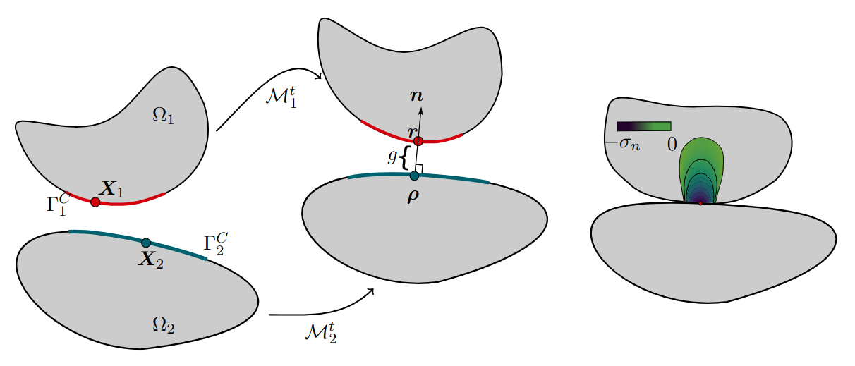
In the next sections, we will define the specific forms of the gap function (\(g_n\)) and contact pressure (\(\lambda_n\)) for contact problems. Let’s consider a point on the surface of one body (we will call it the contactor body) and the surface of another body (we will call it the target body).
The Normal Gap Function (\(g_n\))
The first step is to define the separation between the bodies which will be our inequality constraint.
The normal gap \(g_n\) is the shortest distance from a contactor point \(\boldsymbol{r}\) to the target surface, measured along the normal vector \(\boldsymbol{\rho}\) of the target surface. To define this precisely, we first find the closest-point projection, \(\boldsymbol{r}\), of the contactor point onto the target surface.
The gap is then defined as: \[g_n = (\boldsymbol{r} - \boldsymbol{\rho}) \cdot \boldsymbol{n}\]
where \(\boldsymbol{\rho}\) is the closest-point projection of the contactor point onto the target surface and \(\boldsymbol{n}\) is the normal vector to the target surface.
A positive gap means the bodies are separated, while a negative gap implies penetration.
\(g_n \ge 0\): No interpenetration (physical).
\(g_n < 0\): Interpenetration (unphysical).
The Contact Pressure (\(\lambda_n\))
When bodies are in contact, they exert a force on each other. We define the normal contact pressure \(\lambda_n\) as the magnitude of this force per unit area. In our Lagrange multiplier framework, \(\lambda_n\) is the multiplier that enforces the non-penetration constraint.
With these two quantities, we can state the three fundamental conditions for contact:
No Interpenetration (Primal Feasibility): The gap between the bodies must be greater than or equal to zero. This is the non-negotiable physical constraint. \[g_n \ge 0\]
Repulsive Forces Only (Dual Feasibility): Contact forces can only push, never pull (no adhesion). Therefore, the contact pressure must be compressive, meaning it must be a non-positive value. \[\lambda_n \le 0\]
Complementarity Condition: This is the crucial “switching” condition that makes contact nonlinear. A contact pressure can only exist if the bodies are touching (\(g_n = 0\)). If there is a gap (\(g_n > 0\)), the contact pressure must be zero. These two conditions can be elegantly combined into a single equation: \[\lambda_n \cdot g_n = 0\]
Enforcement of contact constraints
Because of the complementarity condition (\(\lambda_n g_n = 0\)), we don’t know in advance which nodes will be in contact. This “switching” behavior makes contact an inherently nonlinear problem, even if the materials themselves are linear.
To solve this, we must use an iterative procedure to discover the correct set of contacting nodes. This procedure is the active-set strategy that we introduced in the previous lecture. The goal of the loop (Assume → Solve → Check → Update) is to find the set of nodes that correctly satisfies all the KKT conditions upon convergence.
There are various strategies to enforce the KKT conditions within a finite element framework. Each has its own trade-offs between accuracy, computational cost, and ease of implementation. In section Constrained minimization, we have seen two methods to enforce constraints: the penalty method and the Lagrange multiplier method. We will use the same methods to enforce the contact constraints.
Penalty Approach
This is an intuitive and popular method. Instead of enforcing \(g_n \ge 0\) as a strict constraint, we add a penalty energy term to the system’s total potential energy. This term is zero if there is no penetration but adds a large energy penalty if \(g_n < 0\). The penalized potential energy \(\Psi\) is:
\[\Psi = \Psi_{\text{elastic}} + \frac{1}{2} k_\text{pen} \int_{\Gamma_c} \langle -g_n \rangle^2 d\text{A}\]
where \(k_\text{pen}\) is a large penalty stiffness and \(\langle \cdot \rangle\) are Macaulay brackets (meaning \(\langle x \rangle = \max(x, 0)\)). This method is easy to implement but allows for a small amount of penetration and the results depend on the choice of \(k_{pen}\). This method is easy to implement but allows for a small amount of penetration and the results depend on the choice of \(k_{pen}\).
Connection to Active Set: Although it doesn’t solve for \(\lambda_n\) directly, the penalty method still requires an active-set-like check at each step to determine which nodes are currently penetrating (\(g_n < 0\)) and therefore which nodes should have a penalty force applied. The way we do this is by checking if \(g_n < 0\) and if so, we apply a penalty force to the nodes.
Lagrange Multipliers
This method enforces the constraint \(g_n = 0\) exactly. The contact pressure \(\lambda_n\) is introduced as a new, independent degree of freedom in the system. This leads to a saddle-point problem (see Constrained minimization for details on saddle-point problems and how to solve them), which satisfies the KKT conditions perfectly at convergence. However, it increases the size of the system matrix and can introduce numerical instabilities if not handled carefully.
\[\Psi = \Psi_{\text{elastic}} + \int_{\Gamma_c} \lambda_n g_n d\text{A}\]
Connection to Active Set: This is where the active-set strategy is used in its full form. At each iteration, the solver performs the following checks to update the set of active contact constraints:
Check for New Contact (Activation): It checks all nodes not in the active set. If any node is found to be penetrating (\(g_n < 0\)), it is added to the active set for the next iteration.
Check for Release (Deactivation): It checks all nodes currently in the active set. If any node is found to have a tensile (pulling) force (\(\lambda_n > 0\), violating dual feasibility), it is removed from the active set.
The loop continues until a full iteration results in no change to the active set.
Discretization in FEM
The theory above is presented in a continuous sense (integrals over surfaces). In the Finite Element Method, we discretize the problem and define these quantities at specific points.
Nodal Enforcement: The contact constraints are typically enforced at the nodes of one of the meshes. The gap function \(g_n\) and the contact pressure \(\lambda_n\) are calculated for each of these specific nodes. The FEM discretization of the lagrange term becomes:
\[\Psi = \Psi_{\text{elastic}} + \sum_{i \in \Gamma_c} \lambda_{n,i} g_{n,i}A_i\]
where \(A_i\) is the area of the contact node \(i\). Basically we are integrating the lagrange term but over the nodes instead of the surface. This is a easier way to enforce the contact constraints especially when we have to search which nodes are in contact.
Contactor and Target: To manage the calculations, we designate one body’s surface as the contactor and the other as the target. The constraints are then calculated for each node on the contactor surface against the faces of the target surface.
Discrete KKT Conditions: For each potential contact node \(i\), the continuous KKT conditions become a set of algebraic inequalities: \[g_{n,i} \ge 0\] \[\lambda_{n,i} \le 0\] \[\lambda_{n,i} \cdot g_{n,i} = 0\]
The active-set strategy’s goal is to find the set of nodes that satisfies these three rules simultaneously.
Contact between a deformable body and a rigid body
A common simplification in engineering is to model one of the contacting bodies as rigid. This is a good assumption when one body is significantly stiffer than the other (e.g., steel tool on an aluminum workpiece).
A rigid body, by definition, has no internal deformation. It can still undergo rigid body motion (translation and rotation), but its shape and the positions of its surface points relative to each other are fixed. This simplifies the problem because:
The contactor body will be the deformable one.
The target body will be the rigid one.
This assumption significantly simplifies the numerical implementation. Since the target surface geometry is fixed and often known analytically (e.g., a flat line or a perfect circle), we gain several advantages:
Simplified Contact Detection: The search for the closest point projection (\(\boldsymbol{x}_{proj}\)) is performed on a known, unchanging surface.
No Normal Vector Updates: The normal vector \(\boldsymbol{n}\) is constant (for flat surfaces) or can be easily computed at any point. It does not change as the load is applied.
Reduced System Size: We only need to solve for the degrees of freedom of the deformable body.
Hertzian contact: An Analytical Benchmark
This theory, first formulated by Heinrich Hertz in 1881, was one of the first successful analytical solutions to a complex problem in elasticity and remains a cornerstone of mechanical engineering and tribology (Johnson 1987).
The core idea behind the theory is that for non-conforming bodies (like two spheres, or a cylinder on a plane), the deformation under load is highly localized in a small region around the contact point. Outside this small region, the stresses are negligible. This allows the complex geometry of the full bodies to be simplified, approximating them as elastic “half-spaces” whose surfaces are described by quadratic functions. This is a very good approximation for many practical cases as we will see in the in-class exercises.
Assumptions:
Materials are linear elastic, homogeneous, and isotropic.
The contact area is very small compared to the dimensions of the bodies.
Surfaces are continuous and non-conforming (initially touch at a point or along a line).
Contact is frictionless.
Example Case: Deformable Cylinder on a Rigid Half-Space (2D)
This is a classic problem to validate a 2D FEM code. A deformable cylinder of radius \(R\) is pressed into a rigid half-space with a total force \(P\) (per unit length).
The key analytical results are:
Contact Half-Width (\(a\)): The width of the contact zone is given by: \[a = \sqrt{\frac{4PR}{\pi E^{*}}}\]
where \(E^{*}\) is the effective modulus. For a plane strain problem, it’s defined as \(E^{*} = \frac{E}{1 - \nu^2}\).
Pressure Distribution (\(p(x)\)): The contact pressure is not uniform; it follows a semi-elliptical distribution: \[p(x) = p_0 \sqrt{1 - \left(\frac{x}{a}\right)^2} \quad \text{for } |x| \le a\]
Maximum Pressure (\(p_0\)): The peak pressure occurs at the center of the contact zone (\(x=0\)): \[p_0 = \frac{2P}{\pi a}\]
A Note on Contact between Two Deformable Bodies
The most general case is contact between two deformable bodies. This is the next level of complexity, as the geometry of the contact interface is now part of the unknown solution.
When both bodies can deform, the problem becomes more challenging because:
Continuous Contact Detection: The search for contact pairs and the calculation of the gap function \(g_n\) must be performed at every iteration of the nonlinear solver, as the position of all nodes is changing.
Normal Vector Updates: The normal vector \(\boldsymbol{n}\) at the contact point also changes as the target surface deforms. It must be recomputed based on the current, deformed shape.
Symmetric Treatment: The distinction between “contactor” and “target” can become arbitrary, and advanced methods often treat both surfaces symmetrically.
We will explore how to handle these additional complexities in class after mastering the deformable-rigid case.