In-class activity: Active set method

In our last exercise, we used Lagrange multipliers to enforce constraints where the set of constrained nodes, the active set, was known from the start and never changed. This is the case for standard Dirichlet boundary conditions.

But what about more complex problems, like contact or fracture, where we don’t know which parts of a body will be constrained at equilibrium? For this, we need an iterative approach to discover the correct set of active constraints. This is the active-set strategy.

To learn this powerful technique, we will simulate a simple problem: an elastic thin film (length 20 \(m\), height 1 \(m\)) is partially “glued” to a rigid surface. We will then pull it off, and iteratively determine which parts of the glue fail.

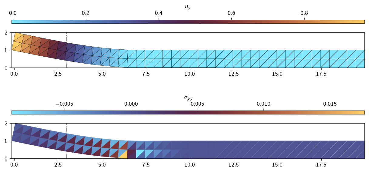
An animation of the debonding process is shown below. The displacement increment for each step is shown in the scalar bar.

The reason why the above physical problem comes under a constraint problem is because of the following reason:

• The nodes of the lower surface are bonded to the rigid surface i.e. the displacement in the \(y\)-direction is constrained to be zero. This can be written as: \[ u^{i}_y = 0, \quad \forall i \in \mathcal{A} \] where \(\mathcal{A}\) is the set of nodes on the lower surface. The constraint equation is given as: \[ g_i(u) = u_y - 0 \]

  We can enforce this constraint by using a Lagrange multiplier \(\lambda_i\) for each node \(i\) in the active set. The \(\lambda_i\) is the force exerted by the adhesive on the node \(i\) in the \(y\)-direction to keep it in place.

  The energy functional thus is given as

  \[ \mathcal{L}(\boldsymbol{u}, \boldsymbol{\lambda}) = \Psi_\text{e}(\boldsymbol{u}) + \sum_{i \in \mathcal{A}} \lambda_i g_i(\boldsymbol{u}) \]

• However, as soon as the force necessary (\(\lambda_i\)) to keep the nodes constrained reaches a critical value (\(\lambda_{crit}\)), the nodes are free to move in the \(y\)-direction. This means that the number of nodes in the active set \(\mathcal{A}\) changes as we keep pulling the bar.

Objective

The goal of this exercise is to:

• Implement an iterative Solve \(\rightarrow\) Check \(\rightarrow\) Update loop, which is the core of any active-set algorithm.
• Use the Lagrange multipliers as physical quantities (adhesive force) to check a failure criterion.
• Simulate how the bonded area of the bar shrinks as the applied load increases.
• Understand the fundamental difference between problems with a fixed active set and those where the active set is part of the solution.

Workflow

For this exercise, the different energy terms are given as follows:

• Elastic energy \(\Psi_\text{e}(\boldsymbol{u})\)
• Lagrange term \(\sum_{i \in \mathcal{A}} \lambda_i g_i(\boldsymbol{u})\)
• Lagrange function \(\mathcal{L}(\boldsymbol{u}, \boldsymbol{\lambda}) = \Psi_\text{e}(\boldsymbol{u}) + \sum_{i \in \mathcal{A}} \lambda_i g_i(\boldsymbol{u})\)

In the above energy functional, finding the correct set of nodes that belong to the active set \(\mathcal{A}\) is the key to solving the problem. Your task is to implement a solver that finds the correct active set \(\mathcal{A}\) for each increment of applied load and then uses it to compute the energy functional.

• Initialization: Define the initial active set \(\mathcal{A}\) as all the nodes that are bonded to the rigid surface at the start.

• Solve: For the current active set \(\mathcal{A}\), solve the KKT system to find the displacements \(\boldsymbol{u}\) and the adhesive forces (Lagrange multipliers) \(\boldsymbol{\lambda}\) for each bonded node.

• Check Condition: For each node \(i\) in the active set, check if its adhesive force has exceeded the critical strength: \[ \text{Is } \lambda_i > \lambda_\text{crit}? \]

• Update Active Set: If the traction at a node is too high, the bond has failed. Remove that node from the active set \(\mathcal{A}\). It is now a free node.

• Repeat: If the active set changed in the last step, you must return to Solve step and resolve the system with the new, smaller active set. The process is converged for the current load step only when an entire solve-check-update loop results in no change to the active set.

import jax

jax.config.update("jax_enable_x64", True)  # use double-precision
jax.config.update("jax_persistent_cache_min_compile_time_secs", 0)
jax.config.update("jax_platforms", "cpu")
import jax.numpy as jnp
from jax import Array

from tatva import Mesh, Operator, element, sparse
from tatva.plotting import STYLE_PATH, colors, plot_element_values, plot_nodal_values


from typing import Callable, Optional, Tuple

from functools import partial
from jax_autovmap import autovmap
import numpy as np

import matplotlib.pyplot as plt

Model setup

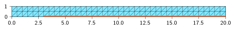
We will generate a mesh for a bar of length 10 and height 2. The bar is meshed with triangles and the adhesive is only on the lower surface.

def generate_block_mesh(
    nx: int,
    ny: int,
    lxs: Tuple[float, float],
    lys: Tuple[float, float],
    curve_func: Optional[Callable[[Array, float], bool]] = None,
    tol: float = 1e-6,
) -> Tuple[Array, Array, Optional[Array]]:
    """
    Generates a 2D triangular mesh for a rectangle and optionally extracts
    1D line elements along a specified curve.

    Args:
        nx: Number of elements along the x-direction.
        ny: Number of elements along the y-direction.
        lxs: Tuple of the x-coordinates of the left and right edges of the rectangle.
        lys: Tuple of the y-coordinates of the bottom and top edges of the rectangle.
        curve_func: An optional callable that takes a coordinate array [x, y] and
                    a tolerance, returning True if the point is on the curve.
        tol: Tolerance for floating-point comparisons.

    Returns:
        A tuple containing:
        - coords (jnp.ndarray): Nodal coordinates, shape (num_nodes, 2).
        - elements_2d (jnp.ndarray): 2D triangular element connectivity.
        - elements_1d (jnp.ndarray | None): 1D line element connectivity, or None.
    """

    x = jnp.linspace(lxs[0], lxs[1], nx + 1)
    y = jnp.linspace(lys[0], lys[1], ny + 1)
    xv, yv = jnp.meshgrid(x, y, indexing="ij")
    coords = jnp.stack([xv.ravel(), yv.ravel()], axis=-1)

    def node_id(i, j):
        return i * (ny + 1) + j

    elements_2d = []
    for i in range(nx):
        for j in range(ny):
            n0 = node_id(i, j)
            n1 = node_id(i + 1, j)
            n2 = node_id(i, j + 1)
            n3 = node_id(i + 1, j + 1)
            elements_2d.append([n0, n1, n3])
            elements_2d.append([n0, n3, n2])
    elements_2d = jnp.array(elements_2d)

    # --- 2. Extract 1D elements if a curve function is provided ---
    if curve_func is None:
        return coords, elements_2d, None

    # Efficiently find all nodes on the curve using jax.vmap
    on_curve_mask = jax.vmap(lambda c: curve_func(c, tol))(coords)

    elements_1d = []
    # Iterate through all 2D elements to find edges on the curve
    for tri in elements_2d:
        # Define the three edges of the triangle
        edges = [(tri[0], tri[1]), (tri[1], tri[2]), (tri[2], tri[0])]
        for n_a, n_b in edges:
            # If both nodes of an edge are on the curve, add it to the set
            if on_curve_mask[n_a] and on_curve_mask[n_b]:
                # Sort to store canonical representation, e.g., (1, 2) not (2, 1)
                elements_1d.append(tuple(sorted((n_a, n_b))))

    if not elements_1d:
        return coords, elements_2d, jnp.array([], dtype=int)

    # return coords, elements_2d, jnp.unique(jnp.array(elements_1d), axis=0)

    mesh = Mesh(coords, elements_2d)

    return (
        mesh,
        jnp.unique(jnp.array(elements_1d), axis=0),
    )

Along with the nodes and the elements associated with the mesh, we also need the nodes and the elements associated with the interface where the adhesive is present.

We assume that the adhesive is only on the lower surface and starts at a distance of 3.0 from the left edge.

We will use the interface_elements variable to store the elements associated with the interface.

The generate_block_mesh function is a helper function that generates the mesh and the interface elements.

Nx = 40  # Number of elements in X
Ny = 2  # Number of elements in Y
Lx = 20  # Length in X
Ly = 1  # Length in Y

adhesive_start = 3. # x position of the start of the adhesive region


# function identifies nodes on the cohesive line at y = 0. and x > 3.0
def interface_line(coord: Array, tol: float) -> bool:
    return jnp.logical_and(jnp.isclose(coord[1], 0.0, atol=tol), coord[0] >= adhesive_start)


(
    mesh,
    interface_elements,
) = generate_block_mesh(
    nx=Nx, ny=Ny, lxs=(0, Lx), lys=(0, Ly), curve_func=interface_line
)

n_nodes = mesh.coords.shape[0]
n_dofs_per_node = 2
n_dofs = n_dofs_per_node * n_nodes

Below we plot the mesh with the adhesive region shown in red.

plt.style.use(STYLE_PATH)
plt.figure(figsize=(6, 3))
ax = plt.axes()
ax.tripcolor(
    mesh.coords[:, 0],
    mesh.coords[:, 1],
    triangles=mesh.elements,
    edgecolors="black",
    linewidths=0.2,
    shading="flat",
    cmap="managua_r",
    facecolors=np.ones(mesh.elements.shape[0]),
)


# Highlight the extracted 1D elements in red
for edge in interface_elements:
    ax.plot(mesh.coords[edge, 0], mesh.coords[edge, 1], colors.red, lw=3)

ax.set_aspect("equal")
ax.margins(0, 0)
plt.show()

Mesh with cohesive elements

Defining the material properties

Let us define the material parameters mainly the Young’s modulus and the Poisson’s ratio.

\[ E = 1.0~ \mathrm{N/m^2}, \quad \nu = 0.3 \]

To calculate the shear modulus and the first Lamé parameter, we use the following formulas:

\[ \mu = \frac{E}{2(1 + \nu)}, \quad \lambda = \frac{E \nu}{(1 + \nu)(1 - 2\nu)} \]

from typing import NamedTuple


class Material(NamedTuple):
    """Material properties for Linear elastic material"""

    mu: float  
    lmbda: float  


E = 1.0
nu = 0.3

mu = E / (2 * (1 + nu))
lmbda = E * nu / ((1 + nu) * (1 - 2 * nu))

mat = Material(mu=mu, lmbda=lmbda)

Define the total elastic energy

\[ \Psi_\text{e}(\boldsymbol{u}) = \frac{1}{2} \int_\Omega \psi_e d\Omega \]

where

\[ \psi_\text{e}(x) = \frac{1}{2} \sigma(x) : \epsilon(x) \]

where \(\sigma\) is the stress tensor and \(\epsilon\) is the strain tensor.

\[ \sigma = \lambda \text{tr}(\epsilon) \mathbf{I} + 2\mu \epsilon \]

and

\[ \epsilon = \frac{1}{2} (\nabla u + \nabla u^T) \]

# --- Material model (linear elasticity: plane strain) ---
tri = element.Tri3()
op = Operator(mesh, tri)


@autovmap(grad_u=2)
def compute_strain(grad_u):
    return 0.5 * (grad_u + grad_u.T)


@autovmap(eps=2, mu=0, lmbda=0)
def compute_stress(eps, mu, lmbda):
    I = jnp.eye(2)
    return 2 * mu * eps + lmbda * jnp.trace(eps) * I


@autovmap(grad_u=2, mu=0, lmbda=0)
def strain_energy(grad_u, mu, lmbda):
    eps = compute_strain(grad_u)
    sigma = compute_stress(eps, mu, lmbda)
    return 0.5 * jnp.einsum("ij,ij->", sigma, eps)


@jax.jit
def total_elastic_energy(u_flat: Array) -> float:
    u = u_flat.reshape(-1, n_dofs_per_node)
    u_grad = op.grad(u)
    energy_density = strain_energy(u_grad, mat.mu, mat.lmbda)
    return op.integrate(energy_density)

compute_internal_force = jax.jacrev(total_elastic_energy)

Defining the dofs for applied displacement

Now we get the dofs for the left edge nodes where we apply the displacement in the \(y-\)direction. The total displacement applied is 1.0m.

\[ u_y^{i} = 1.0 \quad \forall i ~\text{is the dof associated with the nodes on the left edge} \]

Hint

Locate the nodes on the left edge and get the dofs associated with them.

We will use the fixed_dofs variable to store the dofs associated with the left edge nodes.

left_nodes = # get the nodes on the left edge

fixed_dofs = [dofs_associated_with_left_edge_nodes]

n_fixed_dofs = len(fixed_dofs)

applied_disp = 1.0 # total applied displacement

y_max = jnp.max(mesh.coords[:, 1])
y_min = jnp.min(mesh.coords[:, 1])
x_min = jnp.min(mesh.coords[:, 0])
x_max = jnp.max(mesh.coords[:, 0])
height = y_max - y_min


upper_nodes = jnp.where(jnp.isclose(mesh.coords[:, 1], y_max))[0]
lower_nodes = jnp.where(jnp.isclose(mesh.coords[:, 1], y_min))[0]
left_nodes = jnp.where(jnp.isclose(mesh.coords[:, 0], x_min))[0]

fixed_dofs = jnp.concatenate(
    [
        2 * left_nodes + 1,
    ]
)


applied_disp = 1.

prescribed_values = jnp.zeros(n_dofs)
prescribed_values = prescribed_values.at[2 * left_nodes + 1].set(applied_disp)

Defining the dofs for the interface nodes

Since the adhesive is only on the lower surface, we need to extract the dofs associated with the interface nodes. These are the nodes that are on the adhesive line and we will use the interface_elements to extract the dofs associated with the interface nodes.

We will use the interface_dofs variable to store the dofs associated with the interface nodes.

Hint

Get the interface nodes from the interface_elements and then get the dofs associated with them.

interface_nodes = # get unique nodes from the interface_elements

interface_dofs = [dofs_associated_with_interface_nodes]

n_interface_dofs = len(interface_dofs)

interface_nodes = jnp.unique(interface_elements.flatten())
interface_dofs = jnp.concatenate([2 * interface_nodes + 1])

print(interface_dofs)

[ 37  43  49  55  61  67  73  79  85  91  97 103 109 115 121 127 133 139
 145 151 157 163 169 175 181 187 193 199 205 211 217 223 229 235 241]

len(interface_dofs)

35

Defining the constraints

Let us now define the tie constraints. We will use the apply_constraints function to apply the constraints to the nodes of the two surfaces. Along with applying the constraints to the nodes of the two surfaces, we also apply constraints to the dofs of the nodes where Dirichlet boundary conditions are applied.

We have two set of constraints. The first set of constraints corresponds to the adhesive constraints at the interface.

\[ g_i(\boldsymbol{u}) = \boldsymbol{u}_y - \boldsymbol{0} \quad \forall i \in \mathcal{A} \]

where \(\mathcal{A}\) is the set of nodes on the interface

And the second set of constraints corresponds to the displacement constraints at the left edge nodes.

\[ g_i(\boldsymbol{u}) = \boldsymbol{u} - \boldsymbol{u}_0 \quad \forall i \in \mathcal{B} \]

where \(\mathcal{B}\) is the set of nodes on the left edge.

We can now define the apply_constraints function which applies these constraints to the nodes of the two surfaces. We will represents the constraints as a vector of length len(fixed_dofs) where the elements correspond to the displacement constraints.

We will directly apply the interface constraints within the apply_constraints function as it is always constant.

Therefore, the constraints vector is given as:

\[ \boldsymbol{g}(\boldsymbol{u}) = \begin{bmatrix} \boldsymbol{g}_A(\boldsymbol{u}) \\ \boldsymbol{g}_B(\boldsymbol{u}) \end{bmatrix} \]

Hint

The function definition for applying the constraints will look something like this:

def apply_constraints(u, constraints, interface_dofs, fixed_dofs):
    """
    Apply the tie constraints to the nodes of the two surfaces.

    Args:
        u: The displacement vector of the nodes, shape (n_dofs,)
        constraints: The constraints vector, shape (n_fixed_dofs,)
        interface_dofs: The dofs associated with the interface nodes, shape (n_interface_dofs,)
        fixed_dofs: The dofs associated with the left edge nodes, shape (n_fixed_dofs,)

    Returns:
        The constraints vector, shape (n_interface_dofs + n_fixed_dofs,)
    """
    
    # compute the adhesion constraint, g_A(u)
    ...
    
    # compute the applied displacement constraint, g_B(u)
    ...
    
    # combine the two constraints into a single 1D vector
    ...
    
    # return the constraints vector
    return ...

@jax.jit
def tie_constraints(u, constraints, interface_dofs, fixed_dofs):
    u_tie = u[interface_dofs] - y_min
    u_fixed = u[fixed_dofs] - constraints

    return jnp.concatenate([u_tie, u_fixed])


apply_constraints = partial(
    tie_constraints,
    interface_dofs=interface_dofs,
    fixed_dofs=fixed_dofs,
)

Similar to the exercise in Dirichlet BC as constraints (Lagrange multiplier), we can use the jax.jacrev function to automatically compute the Jacobian of the apply_constraints function. Remember that \(\mathbf{B}\) is given as

\[ \mathbf{B} = \frac{\partial \boldsymbol{g}}{\partial \boldsymbol{u}} \]

where \(\boldsymbol{g}\) is the constraint function. We will use this property of \(\mathbf{B}\) to compute it automatically. This could be useful for cases where the constraint function is complex and difficult to compute manually.

Hint

The Jacobian of the apply_constraints function can be computed using the jax.jacrev function.

constraints = jnp.zeros(len(fixed_dofs))
B = jax.jacrev(apply_constraints)(jnp.zeros(n_dofs), constraints).astype(jnp.int32)
nb_cons = B.shape[0]

We can see below the sparsity pattern of the \(\mathbf{B}\) matrix. The non-zero entries are the rows of the \(\mathbf{B}\) matrix that correspond to the constraints applied to the nodes of the interface.

plt.style.use(STYLE_PATH)
plt.figure(figsize=(5, 5))
ax = plt.axes()
ax.spy(B, color=colors.blue, markersize=4)
plt.show()

Figure 9.1: The \(\mathbf{B}\) matrix showing the sparsity pattern due to the tie constraints

Defining the Lagrange functional

Now we can define the Lagrange functional. We will use the jax.jacrev function to compute the gradient and later use the sparsity pattern to compute the sparse stiffness matrix of that gradient.

@jax.jit
def lagrange_functional(z, fext, constraints):
    u = z.at[:-nb_cons].get()
    _lambda = z.at[-nb_cons:].get()

    return (
        total_elastic_energy(u)
        - jnp.vdot(fext, u)
        + jnp.vdot(_lambda, apply_constraints(u, constraints))
    )


dLdz = jax.jacrev(lagrange_functional)

Use sparsity pattern to compute the sparse stiffness matrix of the Lagrange functional. Use the sparse.create_sparsity_pattern_KKT function to create the sparsity pattern and then use the sparse.jacfwd function to compute the sparse stiffness matrix from the gradient.

sparsity_pattern = sparse.create_sparsity_pattern_KKT(
    mesh, n_dofs_per_node=n_dofs_per_node, B=B
)

d2Ldz2_sparse = sparse.jacfwd(dLdz, sparsity_pattern=sparsity_pattern)

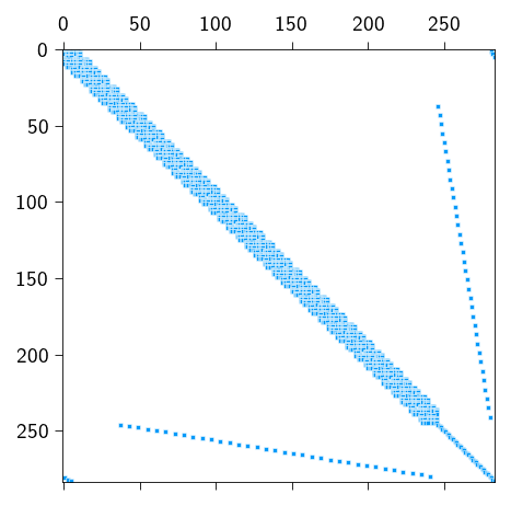
The complete sparsity pattern of the KKT system is shown below. You can see the 4 blocks: the stiffness matrix of the elastic energy, the constraint matrix, its transpose and the Lagrange multiplier matrix.

\[ \begin{bmatrix} \mathbf{K} & \mathbf{B}^T \\ \mathbf{B} & 0 \end{bmatrix} \]

Below you can see the sparsity pattern of the complete KKT system.

plt.style.use(STYLE_PATH)
plt.figure(figsize=(3, 3), layout="constrained")
ax = plt.axes()
ax.spy(sparsity_pattern.todense(), color=colors.blue, markersize=2)
plt.show()

Figure 9.2: The sparsity pattern of the complete KKT system

Critical strength of the adhesive

The critical strength of the adhesive is given by the maximum value of the adhesive traction. For this exercise, we assume that the critical strength is

\[ \lambda_\text{crit} = 10^{-2} ~ \mathrm{N} \]

lambda_crit = 1e-2

Understanding the Sign of λ

In our formulation, the Lagrangian is \(\mathcal{L} = \Psi_e + \lambda g\). Our constraint for the interface is \(g_i(\boldsymbol{u}) = \boldsymbol{u}_y^i - 0\).

When \(g(u) > 0\), to enforce the constraint, the Lagrange multiplier (\(\lambda_i\)) must act as a force in the \(+y\) direction.

A physical tensile (pulling) traction, which is what a adhesive will do, on a node acts in the \(+y\) direction. This means that a physical tensile traction due to the adhesive corresponds to a positive value of \(\lambda_i\). Therefore, the condition “the tensile traction exceeds the critical value” is checked in the code as \(\lambda_i > \lambda_{crit}\).

Let us see why \(\lambda\) must be positive for this problem from two different perspective: a energy perspective and a force perspective.

From Energy Perspective

The system will always try to minimize the total energy \(\mathcal{L}\). Since we are pulling the bar upwards. To lower its elastic energy (\(\Psi_e\)), the bar wants to move in the \(+y\) direction, which would make \(g = u_y > 0\).

The term \(\lambda_i\) must act as a penalty that increases the total energy if the constraint is violated. It must make any upward movement (\(g > 0\)) energetically unfavorable. Therefore, when \(g\) tries to become positive, \(\lambda_i\) must be a positive penalty. This means that \(\lambda_i\) must also be positive.

From Force Perspective

The physical adhesive force, \(F_{adhesive}\), is the force the glue exerts on the bar to hold it down (acting in the \(-y\) direction). This constraint force is derived from the Lagrangian as the negative gradient of the constraint term:

\[ F_{adhesive} = -\frac{\partial (\lambda g)}{\partial u_y} = -\frac{\partial (\lambda u_y)}{\partial u_y} = -\lambda \]

Since the physical adhesive force is pulling down, its scalar value is negative (\(F_{adhesive} < 0\)). Therefore, if \(F_{adhesive} = -\lambda\), then \(\lambda\) must be positive.

The bond fails when the magnitude of the tensile traction exceeds the critical strength: \(\|F_{adhesive}\| > \lambda_{crit}\). Since \(\|\boldsymbol{F}_{adhesive}\| = \|-\boldsymbol{\lambda}\| = \lambda\) (because \(\lambda\) is positive), the correct condition is simply:

\[ \text{Is } \lambda > \lambda_{crit}? \]

The Logic of the Active-Set Strategy

Before we dive into the implementation, let’s understand the logic of the active-set strategy. In our previous exercises with fixed constraints, the size of our KKT system was constant. We built one large matrix and solved it.

In this problem, when a node’s bond fails, its constraint equation and its associated Lagrange multiplier (\(\lambda_i\)) should, in principle, be removed from the problem. This means the KKT matrix should shrink at each iteration. Rebuilding the entire sparse KKT matrix and its sparsity pattern from scratch every time a single node is released would be incredibly inefficient.

Therefore, we need a strategy to handle a system whose size is constantly changing?

The core idea is that instead of rebuilding the matrix, we work with a fixed-size system corresponding to the largest possible active set (all initial interface nodes) and then simply “switch off” the constraints that become inactive.

We will use a boolean array active is for this purpose. It acts as a set of on/off switches for our constraints.

• Physical Meaning: A “switched-off” constraint (active[i] = False) means the glue at that node has failed. Physically, it should exert no force (\(\lambda_i = 0\)) and no longer constrain the node’s displacement.

• Mathematical Implementation: How do we enforce \(\lambda_i = 0\) for an inactive constraint within our large KKT system \(\mathbf{A}\boldsymbol{z} = \boldsymbol{r}\)? We can replace the \(i\)-th constraint equation with the trivial equation:

  \[1 \cdot \lambda_i = 0\]

  We achieve this by modifying the system matrix \(\mathbf{A}\) and the residual vector \(\boldsymbol{r}\):

  • We take the row in \(\mathbf{A}\) corresponding to the inactive \(\lambda_i\) and set all its entries to zero, except for the diagonal entry which we set to 1.
  • We set the corresponding entry in the residual vector \(\boldsymbol{r}\) to 0.

  If you will remember this is the Lifting approach that we used to force the boundary condition in In-class activity: Linear elastic problem. Instead of forcing the displacement to be a certain value, we are forcing the \(\lambda_i\) of the inactive node to be 0.

This trick allows us to use a single, fixed-size system while ensuring that the inactive Lagrange multipliers are correctly driven to zero.

Why is this different from the standard Lagrange multiplier case?

When the active set is fixed (like for standard Dirichlet BCs), we know from the start which constraints are “on”. We build the corresponding KKT system once and solve it. We don’t need an iterative “check and update” loop because the set of rules never changes.

Here, the rules of the game (which nodes are constrained) are part of the solution itself. The active-set loop is the process of discovering these rules. The “zeroing out” strategy (or the Lifting approach) is simply an efficient computational trick to manage this discovery process without costly matrix resizing.

Implementing the active-set strategy

Implement the active set strategy to solve the problem. Since the update of the active-set depends on the solution or evolves with solution, therefore it must be implemented within the Netwon-Solver. So as we solve the system and iterate towards a solution, we keep checking based on the iterative solution, if the active-set is changing.

Therefore, the Newton-Solver is doing two jobs at once:

• it’s finding the equilibrium solution (Newton’s method)
• figuring out which nodes are still glued (the active-set strategy).

Use the newton_sparse_solver function to solve the KKT system and within each iteration, update the active set \(\mathcal{A}\) based on the current adhesive forces.

Hint

Before you start implementing the active set strategy, let’s understand the following:

• The active Array: Our solver now needs to keep track of which constraints are “on” or “off”. The best way to do this is with a new state variable: a boolean array called active of the same size as the number of adhesive constraints. True means the bond is active; False means it has failed.

• A Fixed-Size System: Remember that we are not changing the size of the KKT system. We are “switching off” constraints. This means your solver will always work with the full-size solution vector z (including all potential \(\lambda\)’s) and the full-size KKT matrix K. The “zeroing out” trick is how we manage the on/off state within this fixed-size system.

• The Loop’s Dual Role: The while loop in your Newton solver is now doing two jobs at once:

  • finding the Newton step dz for the current set of active constraints, and
  • updating the active set itself. The system only truly converges when both the residual is small and the active set has stopped changing.

The function newton_sparse_solver would look something like this:

import scipy.sparse as sp

def newton_sparse_solver(z, gradient, hessian, linear_solver=sp.linalg.spsolve):
    """
    Newton solver that includes an active-set strategy for the adhesive constraints.
    """
    iiter = 0
    norm_res = 1.0
    contact_converged = False
    tol = 1e-8
    max_iter = 10 # Increase if needed for more complex debonding

    # TODO Initialize the 'active' array for the adhesive constraints.
    # It should be a boolean array, True for all initially bonded interface nodes.
    # Hint: Its length is len(interface_dofs).
    
    active = jnp.ones(len(interface_dofs), dtype=bool)

    while (norm_res > tol or not contact_converged) and iiter < max_iter:
        # TODO Compute stiffness matrix and residual
        ...

        # Active-Set Modification (Pre-Solve)
        # TODO Find the indices of the inactive lambda DOFs (where 'active' is False)
        ... 
        non_active_idx = .... # contains indices of inactive lambda
        ...

        # TODO Find the row, col indices in sparsity_pattern which contains these non_active_idx
        # we will use these indices to set the entires to 0
        ...
        mask_rows = ... # indices in sparsity_pattern which contain non_active_idx 
        ...

        # TODO FInd the diagonal indices in sparsity pattern which contains non active idx
        # we will use these indices to set the entries to 1.
        ...
        mask_diag = ... #
        ...
        
        # TODO Modifies the matrix stiffness matrix by "zeroing out" rows and setting the diagonal to 1
        ...

        K_data = K_data.at[mask_rows].set(0.0)
        K_data = K_data.at[mask_diag].set(1.0)

        # TODO Build the modified CSR matrix from the modified data.
        ...

        # TODO Modify the residual r by setting entries for inactive constraints to 0
        ...

        # Solve the modified system
        dz = linear_solver(K_modified_csr, residual_modified)
        z = z.at[:].add(dz)

        # Active-Set Update (Post-Solve)
        # TODO Check the deactivation condition and update the active set.
        #  a. Extract the current lambda values for the interface from the updated solution 'z'.
        #  b. Check the condition: (lambda > lambda_crit). This gives a boolean array for newly failed nodes.
        #  c. Check if the active set has converged and set the contact_converged flag to True if it has.
        #  d. Update the main 'active' array. A node can only go from True to False (active &= new_active).
        ...
        
        # TODO Reset lambdas for newly deactivated nodes.
        #  It's crucial to set the lambda values for the nodes that just failed back to 0 in the 'z' vector.
        #  This ensures the next iteration starts from a physically consistent state.
        #  Hint: Use the updated 'active' array and jnp.where.
        ...

        # Convergence Check
        # TODO Calculate the residual norm for convergence.
        #  Remember to re-calculate the full residual based on the updated 'z'.
        #  The residual for the inactive lambda DOFs should be zero before you calculate the norm.
        ...
        
        # TODO manually zero out residual for inactive lambdas before taking the norm
        ...

        print(f"  Residual: {norm_res:.2e}")
        iiter += 1

    return z, norm_res

You’ll notice it’s more complex than a standard Newton solver.

import scipy.sparse as sp


def newton_sparse_solver(z, gradient, hessian, linear_solver=sp.linalg.spsolve):
    """
    Newton solver with sparse linear solver.
    """

    iiter = 0
    norm_res = 1.0
    contact_converged = False

    tol = 1e-8
    max_iter = 10

    active = jnp.ones(len(interface_dofs), dtype=bool)

    while (norm_res > tol or not contact_converged) and iiter < max_iter:
        residual = -gradient(z)

        K = hessian(z)

        not_active = jnp.zeros(K.shape[0], dtype=bool)
        not_active = not_active.at[-nb_cons : -nb_cons + len(interface_dofs)].set(
            ~active
        )
        not_active_idx = jnp.where(not_active)[0]

        mask = jnp.isin(sparsity_pattern.indices, not_active_idx)
        mask_rows = jnp.any(mask, axis=1)

        indices = sparsity_pattern.indices
        mask_diag = jnp.logical_and(
            jnp.isin(indices[:, 0], not_active_idx), indices[:, 0] == indices[:, 1]
        )

        K_data = K.data
        K_data = K_data.at[mask_rows].set(0.0)
        K_data = K_data.at[mask_diag].set(1.0)

        K_csr = sp.csr_matrix((K_data, (K.indices[:, 0], K.indices[:, 1])))

        residual = jnp.where(not_active, 0.0, residual)

        dz = linear_solver(K_csr, residual)
        z = z.at[:].add(dz)

        lambda_solution = z.at[-nb_cons : -nb_cons + len(interface_dofs)].get()

        new_active = jnp.where(lambda_solution > lambda_crit, False, True)
        contact_converged = jnp.all(new_active == active)
        active = active & new_active
        new_lambda = jnp.where(active, lambda_solution, 0.0)

        z = z.at[-nb_cons : -nb_cons + len(interface_dofs)].set(new_lambda)

        residual = -gradient(z)
        residual_at_lambda = jnp.where(
            active, residual.at[-nb_cons : -nb_cons + len(interface_dofs)].get(), 0.0
        )
        residual = residual.at[-nb_cons : -nb_cons + len(interface_dofs)].set(
            residual_at_lambda
        )

        norm_res = jnp.linalg.norm(residual)

        print(f"  Residual: {norm_res:.2e}")

        iiter += 1

    return z, norm_res

Implementing the Incremental Loading Loop

Now that we have the mesh, the energy functions, and the newton_sparse_solver, it’s time to set up the main simulation loop. We will apply the displacement in small increments and solve for equilibrium at each step. This allows us to trace the path of how the debonding progresses as the load increases.

Follow these steps to build the main part of your script.

Hint

Initialization

Before the loop, you need to initialize all the variables for the simulation.

• Create the initial solution vector z_prev, which contains both displacements and Lagrange multipliers. Initialize it as a vector of zeros with the correct total size (n_dofs + nb_cons).
• Initialize the external force vector fext as a vector of zeros.
• Set the number of load increments, n_steps (e.g., 40). We would apply the total applied_disp in n_steps.`
• Calculate the displacement to apply at each step.
• Create several empty Python lists to store the results from each step for later analysis: elastic_energy, load and rnorm_per_step.
  • Here the load is the sum of internal forces (in \(y-\) direction) at the nodes where we applied displacement.

The Main Loading Loop

Create a for loop that iterates through each load step.

for step in range(n_steps):
    print(f"Step {step+1}/{n_steps}")
    # ... Your code for each step will go inside this loop ...

Inside the Loop: Apply Displacement and Prepare Solver

At the beginning of each loop iteration, you need to update the boundary conditions and prepare the functions for the solver.

• Update the constraints vector with the prescribed displacement for the current step.
• Our solver functions (gradient and hessian) require fext and constraints as arguments. To pass them to the solve newton_sparse_solver.

Inside the Loop: Solve for Equilibrium

• Call your newton_sparse_solver function with initial guess.
• Store the new solution in z_new.
• Update the state for the next iteration by setting z_prev = z_new. This is basically providing the solution from the previous step as the initial guess for the next step., which helps the solver converge faster.

Inside the Loop: Post-Processing and Data Storage

After each successful step, calculate and store the physical quantities you want to analyze later.

• Calculate and append the total elastic_energy using the total_elastic_energy function.
• Calculate the total reaction force at the fixed boundary (the “load”) and append it to the load list. You can get this by computing the internal forces and summing the values at the fixed_dofs.
• Store the residual norm for the current step in rnorm_per_step.

After the Loop: Final Solution

Once the loop is complete, extract the final displacement field and Lagrange multipliers from the final z_prev vector for visualization.

z_prev = jnp.zeros(n_dofs + nb_cons)
fext = jnp.zeros(n_dofs)

n_steps = 40

applied_displacement = prescribed_values / n_steps  # displacement increment

lambda_at_interface = []
debonded_area = []
u_per_step = []
elastic_energy = []
load = []
rnorm_per_step = []


for step in range(n_steps):
    print(f"Step {step+1}/{n_steps}")

    constraints = constraints.at[:].set((step + 1) * applied_displacement[fixed_dofs])

    gradient_partial = partial(dLdz, fext=fext, constraints=constraints)
    hessian_sparse_partial = partial(d2Ldz2_sparse, fext=fext, constraints=constraints)

    z_new, rnorm = newton_sparse_solver(
        z_prev,
        gradient=gradient_partial,
        hessian=hessian_sparse_partial,
    )

    z_prev = z_new

    lambda_at_interface.append(z_prev.at[-nb_cons:-nb_cons + len(interface_dofs)].get())
    try:
        idx = np.argwhere(jnp.array(lambda_at_interface[-1]) == 0)[-1][0]
        debonded_area.append(mesh.coords[interface_dofs[idx], 0] - adhesive_start)
    except:
        debonded_area.append(0)

    u_per_step.append(z_prev.at[:n_dofs].get().reshape(n_nodes, n_dofs_per_node))
    elastic_energy.append(total_elastic_energy(u_per_step[-1].flatten()))

    fint = compute_internal_force(u_per_step[-1].flatten())
    load.append(jnp.sum(fint[fixed_dofs]))
    rnorm_per_step.append(rnorm)



u_solution = z_prev.at[:n_dofs].get().reshape(n_nodes, n_dofs_per_node)
lambda_solution = z_prev.at[-nb_cons:-nb_cons + len(interface_dofs)].get()

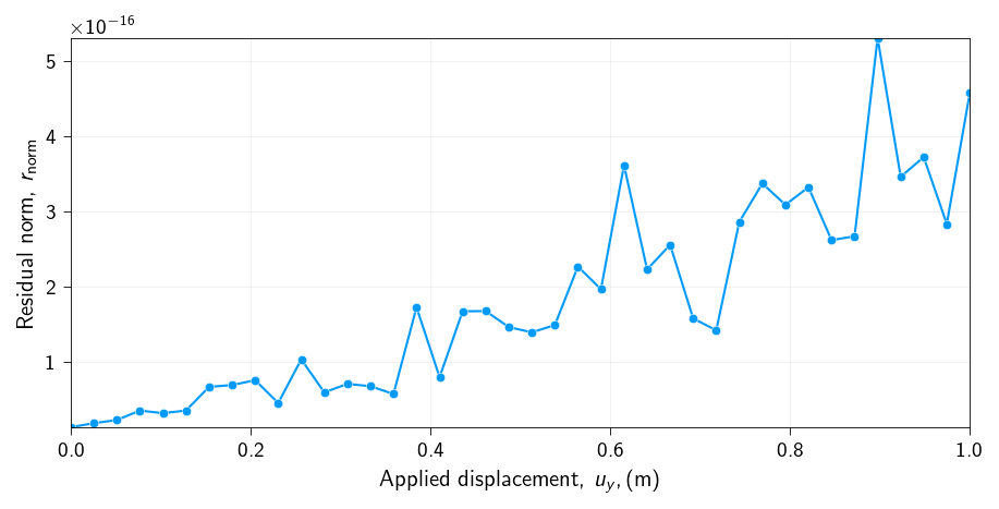
Let us check if the error at each step is below the tolerance level (\(10^{-8}\)) that we specified. We chose to represent the error in the simulation as the norm of the residual.

\[ r_\text{norm} = \| \boldsymbol{r} \| \]

This is important to check because we want to make sure that the solution we are seeing is converged.

plt.style.use(STYLE_PATH)
plt.figure(figsize=(6, 3), layout="constrained")
plt.plot(np.linspace(0, applied_disp, n_steps), rnorm_per_step, 'o-')
plt.xlabel(r"Applied displacement, $u_y, (\mathrm{m})$")
plt.ylabel(r"Residual norm, $r_\mathrm{norm}$")
plt.margins(0, 0)
plt.grid()
plt.show()

Post processing

Now that we have the solution, we can visualize the solution. We will plot the displacements and the stresses in the \(y\)-direction.

# squeeze to remove the quad point dimension (only 1 quad point)
grad_u = op.grad(u_solution).squeeze()
strains = compute_strain(grad_u)
stresses = compute_stress(strains, mat.mu, mat.lmbda)

fig, axs = plt.subplots(2, 1, layout="constrained", figsize=(8, 4))


plot_nodal_values(
    u=u_solution,
    mesh=mesh,
    nodal_values=u_solution[:, 1].flatten(),
    ax=axs[0],
    label=r"$u_y$",
    edgecolors="black",
    shading="flat",
)
axs[0].axvline(adhesive_start, color="gray", lw=1, ls="dashdot", zorder=-10)
axs[0].set_aspect("equal")
axs[0].margins(0.0, 0.0)

plot_element_values(
    u=u_solution,
    mesh=mesh,
    values=stresses[:, 1, 1].flatten(),
    ax=axs[1],
    label=r"$\sigma_{yy}$",
)
axs[1].axvline(adhesive_start, color="gray", lw=1, ls="dashdot", zorder=-10)
axs[1].set_aspect("equal")
axs[1].margins(0.0, 0.0)

plt.show()

Solution from sparse solver

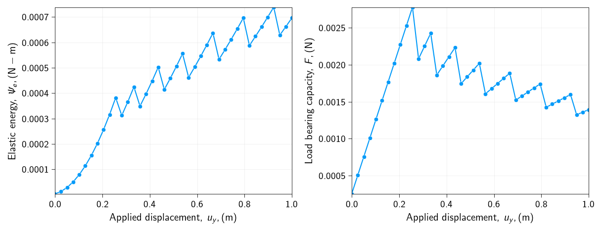
How does the elastic energy and the load bearing capacity of the bar changes with the applied displacement?

Lets us now plot the elastic energy and the load bearing capacity of the bar as a function of the applied displacement.

• What is happening to the elastic energy and the load bearing capacity of the bar as we apply the displacement?

• What is the maximum load bearing capacity of the bar?

• What is the displacement at which the load bearing capacity is reached?

• Why do we see a drop and then a rise in the elastic energy and the load bearing capacity of the bar, after the load bearing capacity is reached?

You will notice in your energy plot that when a node (or a group of nodes) detaches, there is a sudden drop in the total elastic strain energy \(\Psi_e\).

• Where does this energy go?

• Run the simulation with three different values for \(\lambda_{crit}\):

  • a low value (weak glue),
  • a medium value,
  • a very high value (strong glue).

  For the same final applied displacement, how does \(\lambda_\text{crit}\) affect the load bearing capacity and force-displacement curve quantitatively? Explain what this means physically.

• When a node is removed from the active set, the constraint is released instantaneously. How does this snap affect the overall stiffness of the system?

• What happens if you set \(\lambda_{crit} = \infty\)? Which previous problem that we have solved does this simulation become equivalent to? Just describe and nothing to implement.

• Our current model is brittle i.e. the bond at a node is either perfect or it fails completely. What would happen physically if the glue could soften before failing completely i.e. the bond strength would decrease as slowly from \(\lambda_{crit}\) to 0? How might you need to change the active-set algorithm to model this behavior? Just describe and nothing to implement.

plt.style.use(STYLE_PATH)
fig, axes = plt.subplots(1, 2, figsize=(8, 3), layout="constrained")
axes[0].plot(np.linspace(0, applied_disp, n_steps), elastic_energy, 'o-')
axes[0].set_xlabel(r"Applied displacement, $u_y, (\mathrm{m})$")
axes[0].set_ylabel(r"Elastic energy, $\Psi_e, (\mathrm{N-m})$")
axes[0].margins(0, 0)
axes[0].grid()

axes[1].plot(np.linspace(0, applied_disp, n_steps), load, 'o-')
axes[1].set_xlabel(r"Applied displacement, $u_y, (\mathrm{m})$")
axes[1].set_ylabel(r"Load bearing capacity, $F, (\mathrm{N})$")
axes[1].margins(0, 0)
axes[1].grid()
plt.show()

np.max(load)

np.float64(0.0027788056679034817)