Sparse solvers
Until now, we have been working with dense stiffness matrices. What we mean by dense that we store information for each entry of the matrix. Even if the entry is zero, we store it. This is not efficient when we are dealing with problems with a large number of degrees of freedom. Such cases are common in FEM, for example, when we have to refine a mesh around the stress concentration region.
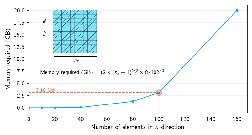
A simple example of how quickly the memory requirement for a dense stiffness matrix grows is given below.
Note
For a mesh with 100 \(\times\) 100 triangular elements (roughly 10000 nodes) with each node having 2 degrees of freedom, the size of a stiffness matrix will be a 20000 \(\times\) 20000 matrix. This means we need to store 400 million entries. And since we need to store each entry in double precision (float64, for accuracy), we need 3.1 GB of memory to store the dense stiffness matrix.
Sparse nature of FEM problems
If we actually look at the stiffness matrix, we will notice is that it is very sparse. By sparsity, we mean that most of the entries are zero. The reason why most of entries are zero is because of the connectivity of the elements (a node of an element is connected to only a few nodes of the neighboring elements) and the fact that interpolation functions (or shape functions) are zero outside of the element. What it means is that a displacement at a node of an element influences only a few of the nodes of the neighboring elements. This is shown in the figure below.

This relation of a node influencing only a few nodes of the neighboring elements gives a banded structure to the stiffness matrix where the non-zero entries are concentrated around a diagonal band. Below we show the stiffness matrix for a 5 \(\times\) 5 mesh. Each row represents a degree of freedom (\(u_x\) or \(u_y\)) and each column also represents a degree of freedom. The non-zero entries are indicated by blue dots. So for each row, a blue dot means that the corresponding degree of freedom is connected to the degree of freedom represented by the column index.
Code: Define mesh for square domain
import jax

jax.config.update("jax_enable_x64", True)  # use double-precision
jax.config.update("jax_persistent_cache_min_compile_time_secs", 0)
jax.config.update("jax_platforms", "cpu")
import jax.numpy as jnp
from jax import Array
from jax_autovmap import autovmap

from tatva import Operator, element
from tatva.plotting import colors

from typing import NamedTuple


class Material(NamedTuple):
    """Material properties for the elasticity operator."""

    mu: float  # Shear modulus
    lmbda: float  # First Lamé parameter


mat = Material(mu=0.5, lmbda=1.0)


@autovmap(grad_u=2)
def compute_strain(grad_u: Array) -> Array:
    """Compute the strain tensor from the gradient of the displacement."""
    return 0.5 * (grad_u + grad_u.T)


@autovmap(eps=2, mu=0, lmbda=0)
def compute_stress(eps: Array, mu: float, lmbda: float) -> Array:
    """Compute the stress tensor from the strain tensor."""
    I = jnp.eye(2)
    return 2 * mu * eps + lmbda * jnp.trace(eps) * I


@autovmap(grad_u=2, mu=0, lmbda=0)
def strain_energy(grad_u: Array, mu: float, lmbda: float) -> Array:
    """Compute the strain energy density."""
    eps = compute_strain(grad_u)
    sig = compute_stress(eps, mat.mu, mat.lmbda)
    return 0.5 * jnp.einsum("ij,ij->", sig, eps)


mesh = Mesh.unit_square(5, 5)
tri = element.Tri3()
op = Operator(mesh, tri)


@jax.jit
def total_energy(u_flat):
    u = u_flat.reshape(-1, 2)
    u_grad = op.grad(u)
    energy_density = strain_energy(u_grad, 1.0, 0.0)
    return op.integrate(energy_density)


K = jax.jacfwd(jax.jacrev(total_energy))(jnp.zeros(mesh.coords.shape[0] * 2))

plt.figure(figsize=(2, 2), layout="constrained")
plt.spy(K, color=colors.blue, markersize=2)
plt.show()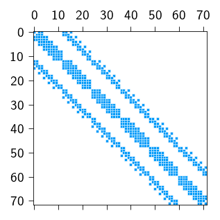
Note
The non-zero entries of the stiffness matrix are concentrated around a diagonal band is indicated by blue dots in the figure above. The zero entries are indicated by white dots.
Therefore, we only need the non-zero entries of the stiffness matrix for solving a mechanical problem, which can save a lot of memory. Since the sparsity pattern (the location of the non-zero entries) is determined by the mesh connectivity (and the local nature of the shape functions), we can create a sparsity pattern for a given mesh and use it to construct a sparse stiffness matrix with only the non-zero entries.
In the section below, we will discuss two aspects of sparse matrices:
- How to store/construct a sparse matrix efficiently?
- How to solve a sparse linear system of equations?
How to store a sparse matrix efficiently?
There are several ways to store a sparse matrix, each designed to save the memory by only storing the non-zero elements. Irrespective of the ways, two things required to store a sparse matrix are:
- The row and column indices of the non-zero elements of a sparse matrix,
(row, col) - The values of the non-zero elements of a sparse matrix,
value
To illustrate the various ways, we will use a simple 4x4 sparse matrix \(\mathbf{K}\) which has 6 non-zero values.
\[ \mathbf{K} = \begin{bmatrix}5 & 0 &0 & 1\\ 0 & 7 & 2 & 0\\ 0 & 0 & 0 & 0 \\ 3 & 0 & 9 & 0 \\ \end{bmatrix} \]
In this course, we will use two ways to sparse matrix based on the what we do with sparse matrices. The two different ways to represent a sparse matrices we will use are:
- Coordinate Format (COO)
- Compressed Sparse Row (CSR)
Coordinate Format (C00)
In this format, sparse matrix is store as a simple list of triplets: (row, col, value). It is the most straightforward way to represent a sparse matrix. For our matrix, the COO representation would be:
row: [0, 0, 1, 1, 3, 3]col: [0, 3, 1, 2, 0, 2]value: [5, 1, 7, 2, 3, 9]
This format is good for building a sparse matrix as it is easy to add new (row, col, value) triplets.
Compressed Sparse Row (CSR)
This format is most often used for performing calculations with sparse matrix. It also uses three arrays to represent a sparse matrix but they have a different meaning:
value: All the non-zero values read from row by row.indices: The column index for each corresponding value in the data array.indptr: Any array of sizenumber of rows + 1. The entryindptr[i]tells the index where the data for rowibegins in thevaluearray. The data for the rowiis located in the slicedata[indptr[i]: indptr[i+1]]
For our matrix, the CSR representation is:
value: [5, 1, 7, 2, 3, 9]indices: [0,3, 1, 2, 0, 2]indptr: [0, 2, 4, 4, 6]
From this we get that:
Row 0starts at index0. The next row starts at index2, so row 0’s data isvalue[0:2]which is[5, 1].Row 1starts at index2. The next row starts at index4, so row 1’s data isvalue[2:4]which is[7, 2].Row 2starts at index4. The next row starts at index4, so row 2’s data isvalue[4:4]which is empty.Row 3starts at index4. The next row starts at index6, so row 3’s data isvalue[4:6]which is[3, 9].
Note
We will both COO and CSR to represent sparse matrices. We will not be constructing these sparse representation ourselves, rather we will use libraries such as scipy to handle this. The above description is just so that you know why we use a specific format for a specific operations.
Constructing sparse stiffness matrix in FEM
In order to construct a sparse stiffness matrix, we need to force the differentiation to be done only on the non-zero entries of the stiffness matrix.
Note
Remember we are using direct differentiation of internal force python to compute the stiffness matrix, therefore, we need to force the differentiation to be done only on the non-zero entries of the stiffness matrix.
\[ \mathbf{K} = \dfrac{\partial \boldsymbol{f}_\text{int}}{\partial \boldsymbol{u}} \]
And to do this, we were using the jax.jacfwd function.
We can force the differentiation to be done only on the non-zero entries of the stiffness matrix if we know the which entries are non-zero and degree of freedom affects the other degree of freedom.
As mentioned earlier, that this information is already available in the mesh connectivity. Therefore, we can use the mesh connectivity to create a sparsity pattern for the matrix which will contain the following information:
(row, col)of the non-zero entries of the stiffness matrix
In tatva, we use the sparse module to create a sparsity pattern for the matrix. The function takes the following arguments:
mesh: The mesh object.n_dofs_per_node: The number of degrees of freedom per node.constraint_elements: Optional array of constraint elements. If provided, the sparsity pattern will be created for the constraint elements.
Note
The constraint_elements is an optional argument. If provided, the sparsity pattern will be created for the constraint elements. We will see an example of this when we discuss fracture mechanics with cohesive elements.
The function returns a jax.experimental.sparse.BCOO object which basically COO representation as we discussed above. The reason we used this format because here we are constructing a sparse representation.
from tatva import sparse

sparsity_pattern = sparse.create_sparsity_pattern(mesh, n_dofs_per_node=2)

plt.figure(figsize=(2, 2), layout="constrained")
plt.spy(sparsity_pattern.todense(), color=colors.blue, markersize=2)
plt.show()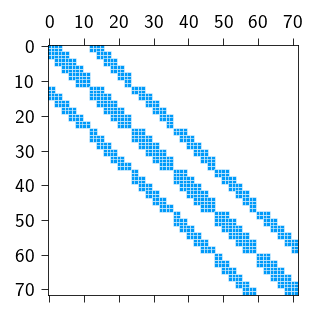
tatva.sparse module based on mesh connectivity
You can access the row, col using the following code:
sparsity_pattern.indices
sparsity_pattern.indicesArray([[ 0, 0],
[ 0, 1],
[ 0, 2],
...,
[71, 69],
[71, 70],
[71, 71]], dtype=int32)Now, we can use the sparsity pattern to create a sparse stiffness matrix. Based on this sparsity pattern, the automatic differentiation is restricted to the non-zero entries of the matrix. This considerably reduces the computational cost. We provided two functions to create a sparse stiffness matrix based on the sparsity pattern: sparse.jacfwd and sparse.jacrev. These functions are wrappers around the jax.jacfwd and jax.jacrev functions, but they take the sparsity pattern as an argument.
K_sparse = sparse.jacfwd(jax.jacrev(total_energy), sparsity_pattern=sparsity_pattern)(
    jnp.zeros(mesh.coords.shape[0] * 2)
)

plt.figure(figsize=(2, 2), layout="constrained")
plt.spy(K_sparse.todense(), color=colors.blue, markersize=2)
plt.show()
We can actually check if the stiffness matrix computed using our sparsity pattern is the same as the stiffness matrix computed using the full matrix.
np.allclose(K_sparse.todense(), K)TrueAs a quick analyses let us check how much memory is saved by using a sparse representation of the stiffness matrix. Below we plot the ratio of the memory required for the sparse stiffness matrix to the memory required for the dense stiffness matrix.
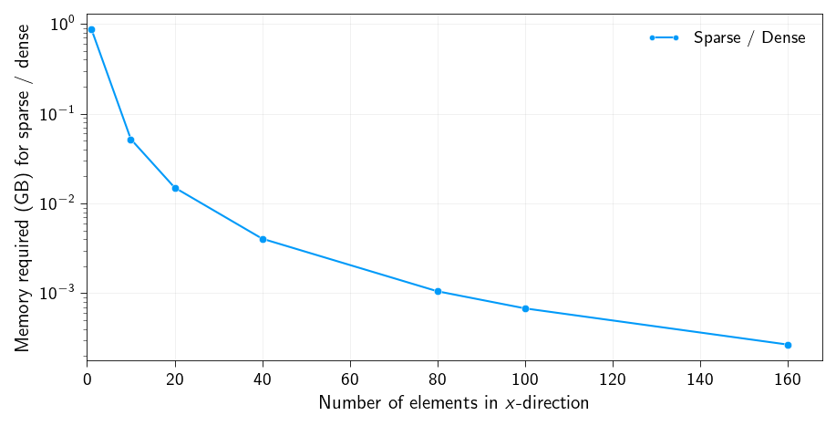
Note
We can clearly see that memory requirement for sparse stiffness matrix decreases tremendously with the number of elements. A reduction of 3 orders of magnitude is seen above.
How to solve a sparse linear system of equations?
Now lets us solve the linear system of equations \(\mathbf{K} \boldsymbol{u} = \boldsymbol{f}\) where \(\mathbf{K}\) is a sparse matrix as we constructed above. For this example, we define a mesh of 50x50 elements and create a function that compute the sparse stiffness matrix for a given displacement field. We will use the functions defined above to construct the sparse stiffness matrix.
mesh = Mesh.unit_square(50, 50)
n_nodes = mesh.coords.shape[0]
n_dofs_per_node = 2
n_dofs = n_nodes * n_dofs_per_node


tri = element.Tri3()
op = Operator(mesh, tri)


@jax.jit
def total_energy(u_flat):
    u = u_flat.reshape(-1, 2)
    u_grad = op.grad(u)
    energy_density = strain_energy(u_grad, 1.0, 0.0)
    return op.integrate(energy_density)


sparsity_pattern = sparse.create_sparsity_pattern(mesh, n_dofs_per_node=n_dofs_per_node)


gradient = jax.jacrev(total_energy)
hessian_sparse = sparse.jacfwd(
    jax.jacrev(total_energy), sparsity_pattern=sparsity_pattern
)
Applying Dirichlet boundary conditions to a sparse stiffness matrix
y_max = jnp.max(mesh.coords[:, 1])
y_min = jnp.min(mesh.coords[:, 1])
x_max = jnp.max(mesh.coords[:, 0])
x_min = jnp.min(mesh.coords[:, 0])

left_nodes = jnp.where(jnp.isclose(mesh.coords[:, 0], x_min))[0]
right_nodes = jnp.where(jnp.isclose(mesh.coords[:, 0], x_max))[0]
fixed_dofs = jnp.concatenate(
    [
        2 * left_nodes,
        2 * left_nodes + 1,
        2 * right_nodes,
    ]
)

prescribed_values = jnp.zeros(n_dofs).at[2 * right_nodes].set(0.3)
To apply the Dirichlet boundary conditions, we use the same lifting approach as we used in In-class activity: Linear elastic problem. This is a constraint approach where the entry of the stiffness matrix corresponding to the constrained degrees of freedom are set to 1 and the corresponding rows and columns are set to 0. In order to do this, we need to know the indices (row, col) of the non-zero entries of the stiffness matrix. Once we have the indices, we can set the corresponding entries to 1 and 0.
We will use the function sparse.get_bc_indices to get the indices of the non-zero entries of the stiffness matrix. The function get_bc_indices takes the following arguments:
sparsity_pattern: The sparsity pattern created using thecreate_sparsity_patternfunction.fixed_dofs: The degrees of freedom where we apply the Dirichlet boundary conditions.
The function returns two arrays:
zero_indices: The indices of the sparsity pattern that correspond to location where the stiffness matrix is set to 0.one_indices: The indices of the sparsity pattern that correspond to location where the stiffness matrix is set to 1.
zero_indices, one_indices = sparse.get_bc_indices(sparsity_pattern, fixed_dofs)Now, we have everything we need to solve the linear system of equations.
Sparse solvers (using SciPy)
We will use SciPy to solve the sparse linear system of equations.
import scipy.sparse as spWe define a newton solver that uses Scipy to solve the linear system of equations. We make use of the sparsity pattern to construct the linear system of equations. Notice that we have to convert the BCOO matrix to a CSR matrix. As we discussed CSR format is the more efficient format for performing mathematical operations on a sparse matrix, therefore, we convert the COO format to CSR format first and then use that CSR format to to solve the linear system.
Scipy has a functionality to construct a CSR matrix from the list of triplets (row, col, value). We use this to first construct the CSR matrix and then use the scipy.linalg.spsolve module to solve
\[ \mathbf{K}\boldsymbol{u} = \boldsymbol{f}_\text{ext} - \boldsymbol{f}_\text{int} \]
The below function implements all these steps.
def newton_scipy_solver(
    u,
    fext,
    gradient,
    hessian_sparse,
    fixed_dofs,
    zero_indices,
    one_indices,
):
    fint = gradient(u)

    iiter = 0
    norm_res = 1.0

    tol = 1e-8
    max_iter = 10

    while norm_res > tol and iiter < max_iter:
        residual = fext - fint
        residual = residual.at[fixed_dofs].set(0.0)

        K_sparse = hessian_sparse(u)
        K_data_lifted = K_sparse.data.at[zero_indices].set(0)
        K_data_lifted = K_data_lifted.at[one_indices].set(1)

        K_csr = sp.csr_matrix(
            (K_data_lifted, (K_sparse.indices[:, 0], K_sparse.indices[:, 1]))
        )

        du = sp.linalg.spsolve(K_csr, residual)
        u = u.at[:].add(du)

        fint = gradient(u)
        residual = fext - fint
        residual = residual.at[fixed_dofs].set(0)
        norm_res = jnp.linalg.norm(residual)

        print(f"  Residual: {norm_res:.2e}")

        iiter += 1

    return u, norm_res
Now, we use the above defined function to solve the problem in 10 loading steps.
u_prev = jnp.zeros(n_dofs)
fext = jnp.zeros(n_dofs)

n_steps = 10

applied_displacement = prescribed_values / n_steps  # displacement increment
for step in range(n_steps):
    print(f"Step {step + 1}/{n_steps}")
    u_prev = u_prev.at[fixed_dofs].add(applied_displacement[fixed_dofs])

    u_new, rnorm = newton_scipy_solver(
        u_prev,
        fext,
        gradient,
        hessian_sparse,
        fixed_dofs,
        zero_indices,
        one_indices,
    )

    u_prev = u_new

u_solution = u_prev.reshape(n_nodes, n_dofs_per_node)
Post-processing
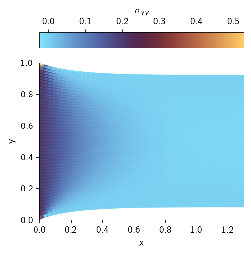
Now we can plot the stress distribution and the displacement.
Code: Plotting the stress distribution
# squeeze to remove the quad point dimension (only 1 quad point)
grad_u = op.grad(u_solution).squeeze()
strains = compute_strain(grad_u)
stresses = compute_stress(strains, mat.mu, mat.lmbda)

plt.figure(figsize=(4, 3), layout="constrained")
ax = plt.axes()
plot_element_values(
    u=u_solution,
    mesh=mesh,
    values=stresses[:, 1, 1].flatten(),
    label=r"$\sigma_{yy}$",
    ax=ax,
)
ax.set_xlabel(r"x")
ax.set_ylabel(r"y")
ax.set_aspect("equal")
ax.margins(0, 0)
plt.show()