Constrained minimization
Constrained problems are a class of optimization problems where the solution to a minimization problem is required to satisfy a set of additional conditions or constraints. Many problems in solid mechanics fall into this category.
- Contact Mechanics: Bodies must not penetrate each other.
- Fracture Mechanics: A crack, once formed, cannot heal itself (an irreversibility constraint).
- Multiphysics: The pressure in a porous solid cannot fall below a physical limit.
In all these cases, a physical process forces the solution to satisfy certain conditions. In fact, a very common example of a constrained problem is the application of Dirichlet boundary conditions. When we prescribe a displacement, we are constraining a degree of freedom to a specific value. Because these problems are so common, it’s essential to have a robust mathematical framework to solve them.
General formulation of constrained problems
Irrespective of the application, a constrained problem can be written as:
\[ \min_{\boldsymbol{u}} \Psi(\boldsymbol{u}) \]
\[ \text{such that} \quad g_i(\boldsymbol{u}) \geq 0 \quad \forall i \in \mathcal{A} \]
where \(\Psi(\boldsymbol{u})\) is the total potential energy of the system, \(g_i(\boldsymbol{u})\) is the i-th constraint function, and \(\mathcal{A}\) is the set of indices for all degrees of freedom that are potentially constrained. The constraint function \(g_i(\boldsymbol{u})\) is also called the inequality constraint.
Note
A constraint \(i\) is said to be active if \(g_i(\boldsymbol{u})=0\) and inactive if the strict inequality \(g_i(\boldsymbol{u}) > 0\) holds. The set of all active constraints is called the active set \(\mathcal{A}\).
Sometimes, the constraints are also equality constraints i.e. \(g_i(\boldsymbol{u}) = 0\). In this case, the constraint function \(g_i(\boldsymbol{u})\) is also called the equality constraint. The constrained problem then can be written as:
\[ \min_{\boldsymbol{u}} \Psi(\boldsymbol{u}) \]
\[ \text{such that} \quad g_i(\boldsymbol{u}) = 0 \quad \forall i \in \mathcal{A} \]
Solving the constrained problem (with either inequality or equality constraints) requires two key ingredients:
A mathematical definition for each constraint function \(g_i\).
An algorithm to determine the active set, since we often don’t know in advance which constraints will be active at equilibrium.
Note
For details on the mathematical formulation of constrained problems, you also refer to Chapter 16 on quadratic programming from (Nocedal and Wright 2006).
Methods to solve constrained problems
There are several techniques to solve constrained problems. The most common are:
- Penalty method
- Lagrange multiplier method
- Augmented Lagrangian method
In this course, we will focus on two methods mainly penalty method and Lagrange multiplier method.
Penalty formulation
In penalty formulation, we convert a constrained problem into an unconstrained problem by adding a penalty energy term to the objective function to enforce the constraint. This new term is designed to be zero if the constraint is satisfied, but grows very large if the constraint is violated.
The penalized energy functional \(\Psi_p(\boldsymbol{u})\) is given by: \[ \Psi_p(\boldsymbol{u}) = \Psi(\boldsymbol{u}) + \Psi(g(\boldsymbol{u}_i)) \]
where \(\Psi(g(\boldsymbol{u}_i))\) is the energy associated with the constraint. The penalty energy term is given by:
\[ \Psi(g(\boldsymbol{u}_i)) = \int_{\Omega_{\mathcal{C}}} \frac{1}{2} \kappa \langle g(\boldsymbol{u}_i)\rangle^2 ~\text{d}\Omega \]
where
- \(\kappa\) is the penalty parameter
- \(\Omega_{\mathcal{C}}\) is the domain (set of nodes or set of elements) where the constraints are expected.
- \(\Big\langle \star\Big\rangle\) is the Macaulay bracket, defined as \[ \Big\langle g(\boldsymbol{u}_i)\Big\rangle = \begin{cases} g(\boldsymbol{u}_i) & \text{if } g(\boldsymbol{u}_i) < 0 \\ 0 & \text{if } g(\boldsymbol{u}_i) \geq 0 \end{cases} \]
this means, that the \(\Big\langle g(\boldsymbol{u}_i)\Big\rangle\) is non-zero only when \(g(\boldsymbol{u}_i) < 0\) i.e. the constraint is violated.
If we look at the energy functional for the constraint, it is very similar to the energy functional for a spring. To make an analogy to a spring, \(\kappa\) will be the spring constant and \(g(\boldsymbol{u}_i)\) will be analogous to the displacement of the spring. As soon as the \(g(\boldsymbol{u}_i)\) becomes negative i.e. the constraint is violated, the spring deforms and will try to restore the original length of the spring which is the constraint being satisfied i.e. \(g(\boldsymbol{u}_i) = 0\). Thus the penalty method is a way to adding a spring to every nodes or elements where the constraint is active and the penalty parameter \(\kappa\) then governs how strongly the spring will try to restore the constraint. A large value of \(\kappa\) will make the spring very stiff and will try to restore the constraint very strongly. A small value of \(\kappa\) will make the spring very flexible and will not try to restore the constraint as strongly.
Based on the above arguments, the new energy functional is given as:
\[ \Psi_p(\boldsymbol{u}) = \Psi(\boldsymbol{u}) + \int_{\Omega_{\mathcal{C}}} \frac{1}{2} \kappa \Big\langle g(\boldsymbol{u}_i)\Big\rangle ^2 ~\text{d}\Omega. \]
Now, we solve by minimizing this new functional in an unconstrained manner:
\[ \frac{\partial \Psi_p}{\partial \boldsymbol{u}} = \mathbf{0} \implies (\mathbf{K}\boldsymbol{u} - \boldsymbol{f}_{\text{ext}}) + \kappa \langle g(\boldsymbol{u}_i)\rangle \boldsymbol{e}_i = \mathbf{0} \]
where \(\mathbf{K}\boldsymbol{u}\) is the internal force vector and \(\boldsymbol{f}\) is the external force vector. \(\boldsymbol{e}_i\) is a vector of all zeros except for a 1 at the \(i\) th position where the constraint is active. \(g(\boldsymbol{u}_i)\) is the value of the constraint at the \(i\) th position.
Rearranging this gives:
\[ (\mathbf{K} + \kappa \boldsymbol{e}_i \boldsymbol{e}_i^T)\boldsymbol{u} = \boldsymbol{f}_{\text{ext}} + \kappa \langle g(\boldsymbol{u}_i)\rangle \boldsymbol{e}_i \]
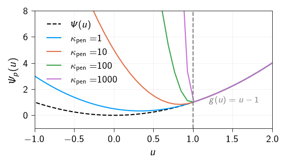
Let us demonstrate the penalty formulation for constrained minimization. We consider a simple example of a spring with one degree of freedom. The potential energy of the system is given by: \[ \Psi(\boldsymbol{u}) = \frac{1}{2} k u^2 \] where \(k\) is the stiffness of the system. The minimum of the potential energy or the equilibrium state of the system is at \(u = 0\).
Now, we impose a constraint that the displacement should be greater than or equal to 1. Hence the constraint function is given by: \[ g(\boldsymbol{u}) = u - 1 \]
The new potential energy functional using the penalty formulation is given by:
\[ \Psi_p(\boldsymbol{u}) = \Psi(\boldsymbol{u}) + \frac{1}{2} \kappa_\text{pen} \Big\langle g(\boldsymbol{u}_i)\Big\rangle ^2 \]
Below, we plot the potential energy functional for the penalty method for different values of the penalty parameter \(\kappa_\text{pen}\). As can be seen, as the penalty parameter increases, the potential energy functional becomes more and more steep and the equilibrium state (minimum of the potential energy functional) of the system shifts towards \(u = 1\) from the original equilibrium state at \(u = 0\).
Ill conditioning
A major drawback of the penalty method is that it introduces numerical ill-conditioning. To approximate the “hard” constraint accurately, the penalty parameter \(\kappa\) must be very large. This creates a large difference in magnitude between the entries of the stiffness matrix \(\mathbf{K}\) and the penalty stiffness \(\kappa\). The resulting system matrix has a very high condition number, which can make it extremely difficult for iterative solvers (like Conjugate Gradient) to converge.
Lagrangian Formulation
The Lagrange multiplier method is a powerful tool that converts a constrained problem into an unconstrained one by introducing new variables, called Lagrange multipliers (\(\lambda\)). For inequality constraints, the full set of conditions for a minimum are known as the Karush-Kuhn-Tucker (KKT) conditions.
We define a new functional called the Lagrangian functional \(\mathcal{L}(\boldsymbol{u}, \lambda)\) as:
\[\mathcal{L}(\boldsymbol{u}, \lambda) = \Psi(\boldsymbol{u}) + \lambda g(\boldsymbol{u}_i)\]
The solution is a stationary point of this Lagrangian that also satisfies the KKT conditions:
Stationary point: \(\frac{\partial \mathcal{L}}{\partial \boldsymbol{u}} = \mathbf{0}\)
Primal feasibility: \(g_i(\boldsymbol{u}) \ge 0\) (The original constraints)
Dual feasibility: \(\lambda_i \le 0\) (Multipliers are non-positive)
Complementarity condition: \(\lambda_i g_i(\boldsymbol{u}) = 0\) (Either the constraint is active, or the multiplier is zero)
The multiplier \(\lambda_i\) has a clear physical meaning: it is the contact or reaction force required to enforce the constraint. The complementarity condition states that this reaction force can only exist if the constraint is active (\(g_i=0\)).
Finding the stationary point of the Lagrangian leads to a saddle-point problem. We are seeking a point that is a minimum with respect to \(\boldsymbol{u}\) and a maximum with respect to \(\boldsymbol{\lambda}\). When discretized, this leads to a system matrix with a characteristic block structure:
\[\begin{bmatrix} \mathbf{A} & \mathbf{B}^{T} \\ \mathbf{B} & \mathbf{C} \end{bmatrix} \begin{Bmatrix} \boldsymbol{u} \\ \lambda \end{Bmatrix} = \begin{Bmatrix} \boldsymbol{f} \\ g \end{Bmatrix}\]
where
\[ \mathbf{A} = \frac{\partial^2 \mathcal{L}}{\partial \boldsymbol{u}^2} = \frac{\partial^2 \Psi}{\partial \boldsymbol{u}^2}, \quad \mathbf{B} = \frac{\partial^2 \mathcal{L}}{\partial \boldsymbol{u} \partial \lambda}, \quad \mathbf{C} = \frac{\partial^2 \mathcal{L}}{\partial \lambda^2} = \mathbf{0} \] and
\[ \boldsymbol{f} = \frac{\partial \mathcal{L}}{\partial \boldsymbol{u}}, \quad g = \frac{\partial \mathcal{L}}{\partial \lambda} \]
Since \(\mathcal{L}\) is linear in \(\lambda\), \(\mathbf{C}\) is a \(\mathbf{0}\) matrix which gives the classic block structure of a saddle-point problem where one of the main diagonal blocks is zero. \[ \begin{bmatrix} \mathbf{A} & \mathbf{B}^{T} \\ \mathbf{B} & \mathbf{0} \end{bmatrix} \begin{Bmatrix} \boldsymbol{u} \\ \lambda \end{Bmatrix} = \begin{Bmatrix} \boldsymbol{f} \\ g \end{Bmatrix} \]
This makes the system matrix indefinite and therefore, the system is not positive-definite.
Let consider the same example as before. The Lagrangian is given by:
\[ \mathcal{L}(\boldsymbol{u}, \lambda) = \frac{1}{2}\kappa u^2 + \lambda \langle u - 1 \rangle \]
Figure 6.2 shows the Lagrangian functional for the constrained spring problem. The stationary point is at the saddle point of the energy landscape (indicated by the white dot). As can be seen, using lagrangian multiplier method, makes the energy landscape non-smooth.
Direct solution of the KKT system
The KKT matrix has a symmetric but indefinite structure (due to the zero block on the diagonal), meaning it has both positive and negative eigenvalues. Because of this, a standard Cholesky factorization (\(\mathbf{A} = \mathbf{L}\mathbf{L}^T\)), which is highly efficient for positive-definite matrices, will fail.
Instead, you must use a solver that can handle indefinite systems.
A general LU decomposition will work correctly as it makes no assumptions about the matrix properties.
A more efficient choice is a specialized factorization for symmetric indefinite matrices like LDLT factorization (\(\mathbf{A} = \mathbf{L}\mathbf{D}\mathbf{L}^T\)). It is roughly twice as fast as LU decomposition and more memory-efficient because it exploits the matrix’s symmetry.
Tip
In this course, we will use the direct solver from either scipy.sparse.linalg or scipy.linalg to solve the KKT system which uses a LU decomposition.
Iterative solution of the KKT system
Iterative solvers are an excellent choice for large-scale KKT systems, especially in 3D, because they are far more memory-efficient than direct solvers and can be faster.
However, the choice of solver is critical. Since the KKT matrix is symmetric but indefinite, the standard Conjugate Gradient (CG) method will not work and may lead to divergence or errors.
You must use an iterative method designed for indefinite systems. The most common choices from the family of Krylov subspace methods are:
MINRES (Minimum Residual Method): This is often the ideal choice. It is designed specifically for symmetric indefinite systems and is analogous to the CG method for this class of problems.
GMRES (Generalized Minimum Residual Method): This robust solver works for any general non-singular matrix. While it will solve the KKT system, it can be less efficient than MINRES as it does not exploit the matrix’s symmetry.
For any iterative method to perform well, a good preconditioner is almost always essential to accelerate convergence. Designing effective preconditioners for such saddle-point systems is a key part of advanced computational mechanics.
Tip
In this course, we will not use the iterative solver for solving the KKT system. The information given here is for your reference only.
Dirichlet Boundary Conditions as a Constrained Problem
In this section, we will see how to apply the penalty method and the Lagrange multiplier method to solve the Dirichlet boundary conditions as a constrained problem. For simplicity, we will apply Dirichlet boundary conditions to a single degree of freedom \(u_i = \bar{u}\). And therefore, the constraint function is:
\[ g(u_i) = u_i - \bar{u} = 0 \] where \(\bar{u}\) is the prescribed displacement at the \(i\)th degree of freedom. If you notice, that the constraint function here is an equality i.e the nodes where constraints is active is already known. This is the reason why we were able to solve the linear elasticity problem just by applying the Dirichlet boundary condtions through the lifting approach. Imagine, if the constraint function had been an inequality i.e the nodes were the ones where the constraint is active were not known, then we cannot apply the lifting approach. And this inequality (or unknown active nodes) actually makes the problem non-linear and therefore, require sophisticated algorithms or approaches to solve.
Thus, the constrained problem can be written as:
\[ \min_{\boldsymbol{u}} \Psi(\boldsymbol{u}) \]
\[ \text{such that} \quad g_i(u) = u_i - \bar{u} = 0 \quad \forall i \in \mathcal{A} \]
Below, we will see how to apply the penalty method and the Lagrange multiplier method to solve the Dirichlet boundary conditions as a constrained problem.
Applying the penalty method
Using penalty method the energy functional becomes:
\[\Psi_p(\boldsymbol{u}) = \Psi(\boldsymbol{u}) + \int_{\Omega_{\mathcal{C}}} \frac{1}{2} \kappa \Big\langle g(u_i)\Big\rangle ^2 ~\text{d}\Omega.\]
In the above equation, we replace the constraint function with the condition $ _i - {u}$ and since the nodes where constraints is active are already known, we can replace the integral with a sum over the nodes where constraints is active.
\[\Psi_p(\boldsymbol{u}) = \Psi(\boldsymbol{u}) + \sum_{i \in \mathcal{C}} \frac{1}{2} \kappa \Big\langle u_i - \bar{u}\Big\rangle ^2\]
Now, we solve by minimizing this new functional in an unconstrained manner:
\[\frac{\partial \Psi_p}{\partial \boldsymbol{u}} = \mathbf{0} \implies (\mathbf{K}\boldsymbol{u} - \boldsymbol{f}_{\text{ext}}) + \kappa(u_i - \bar{u})\boldsymbol{e}_i = \mathbf{0}\]
where
- \(\kappa\) is the penalty parameter
- \(\boldsymbol{e}_i\) is a vector of all zeros except for a 1 at the \(i\) th position where the constraint is active.
Rearranging this gives: \[(\mathbf{K} + \kappa \boldsymbol{e}_i \boldsymbol{e}_i^T)\boldsymbol{u} = \boldsymbol{f}_{\text{ext}} + \kappa\bar{u}\boldsymbol{e}_i\]
Let’s look at the modified stiffness matrix \(\mathbf{K}' = (\mathbf{K} + \kappa \boldsymbol{e}_i \boldsymbol{e}_i^T)\). The matrix \(\boldsymbol{e}_i \boldsymbol{e}_i^T\) is a matrix of all zeros except for a 1 at the diagonal position \((i, i)\). Therefore, this method is equivalent to adding a very large number (\(\kappa\)) to the diagonal element of the stiffness matrix corresponding to the constrained degree of freedom. The modified system to solve is:
\[ \begin{bmatrix} \mathbf{K}_{ff} & \mathbf{K}_{fi} \\ \mathbf{K}_{if} & \mathbf{K}_{ii} + \kappa \end{bmatrix} \begin{Bmatrix} \boldsymbol{u}_f \\ \boldsymbol{u}_i \end{Bmatrix} = \begin{Bmatrix} \boldsymbol{f}_{\text{ext, f}} \\ \boldsymbol{f}_{\text{ext, i}} + \kappa\bar{u} \end{Bmatrix} \]
Tip
If you are familiar with the approach of applying Dirichlet boundary conditions by adding a large number to the diagonal element of the stiffness matrix corresponding to the constrained degree of freedom, then actually you have been using the penalty method without knowing it.
Applying the Lagrange multiplier method
The Lagrangian combines the original potential energy with the constraint equation:
\[ \mathcal{L}(\boldsymbol{u}, \lambda) = \Psi(\boldsymbol{u}) + \boldsymbol{\lambda}\cdot{} g(\boldsymbol{u}) = \left(\frac{1}{2}\mathbf{K}\boldsymbol{u}^2 - \boldsymbol{f}_{\text{ext}}\boldsymbol{u}\right) + \lambda (u_i - \bar{u}) \]
The solution is found at the stationary point of the Lagrangian, where the gradient with respect to all variables (\(\boldsymbol{u}\) and \(\boldsymbol{\lambda}\)) is zero i.e.
\[ \begin{Bmatrix} \frac{\partial \mathcal{L}}{\partial \boldsymbol{u}} \\ \frac{\partial \mathcal{L}}{\partial \boldsymbol{\lambda}} \end{Bmatrix} = \mathbf{0} \]
In the above equation,
\(\frac{\partial \mathcal{L}}{\partial \boldsymbol{\lambda}} = \boldsymbol{0}\) simply recovers the constraint equation: \[ \boldsymbol{u} - \bar{\boldsymbol{u}} = \boldsymbol{0} \implies \boldsymbol{u} = \bar{\boldsymbol{u}} \]
\(\frac{\partial \mathcal{L}}{\partial \boldsymbol{u}} = \mathbf{0}\) gives the original equilibrium equation plus a new term related to the constraint: \[ \mathbf{K}\boldsymbol{u} - \boldsymbol{f}_{\text{ext}} + \boldsymbol{\lambda} \bar{u} \boldsymbol{e}_i = \mathbf{0} \] where \(\boldsymbol{e}_i\) is a vector with a 1 at the \(i\) th position and zeros elsewhere.
Putting these two results together, we get an augmented system of linear equations:
\[\begin{bmatrix} \mathbf{K} & \boldsymbol{e}_i \\ \boldsymbol{e}_i^T & 0 \end{bmatrix} \begin{Bmatrix} \boldsymbol{u} \\ \boldsymbol{\lambda} \end{Bmatrix} = \begin{Bmatrix} \boldsymbol{f}_{\text{ext}} \\ \bar{\boldsymbol{u}} \end{Bmatrix}\]
Our goal is to find the displacement vector \(\boldsymbol{u}\) and the Lagrange multiplier \(\boldsymbol{\lambda}\) (the reaction force). This system is larger (\(n+1 \times n+1\)) and the augmented matrix is not positive-definite due to the zero on the diagonal, which can be inefficient or problematic for certain solvers. As mentioned earlier, we can solve such systems using the direct solver with LU decomposition from scipy.sparse.linalg or scipy.linalg.
References
Nocedal, Jorge, and Stephen J Wright. 2006. Numerical Optimization. Springer.
Yastrebov, Vladislav. 2013. Numerical Methods in Contact Mechanics. Wiley.