In-class activity: Cohesive zone modelling

In this notebook, we will implement a cohesive element in the finite element method. We will use a single cohesive element to understand in detail:

how to implement a cohesive zone approach?
how the traction-separation law is implemented?
how different traction-separation laws affect response of the fracture process?
how a cohesive element behaves when it is subjected to a Mode I loading?

For a solid body undergoing a fracture process, the total potential energy is given by:

\[ \Psi = \Psi_\text{elastic} - \Psi_\text{external} + \Psi_\text{fracture} \]

where \(\Psi_\text{elastic}\) is the elastic energy, \(\Psi_\text{external}\) is the work done by the external forces, and \(\Psi_\text{fracture}\) is the fracture energy that is dissipated in creating new fracture surfaces.

In cohesive zone modelling, we estimate the fracture energy is given by:

\[ \Psi_\text{fracture} = \int_{\Gamma_{coh}} \psi(\delta) \text{d}a \]

where \(\psi(\delta)\) is the work done per unit area in separating the two surfaces of the cohesive zone by an amount \(\delta\). In this exercise, we will make use of different Traction-Separation Laws (TSL) to understand how different TSLs affect the response of the cohesive element.

Lets start with importing the necessary libraries and modules.

Code: Importing the essential libraries

import jax

jax.config.update("jax_enable_x64", True)  # use double-precision
jax.config.update("jax_persistent_cache_min_compile_time_secs", 0)
jax.config.update("jax_platforms", "cpu")
import jax.numpy as jnp
from jax import Array


from tatva import Mesh, Operator, element
from tatva.plotting import STYLE_PATH, colors, plot_nodal_values


from jax_autovmap import autovmap
import numpy as np


from typing import NamedTuple


import matplotlib.pyplot as plt

Model Setup

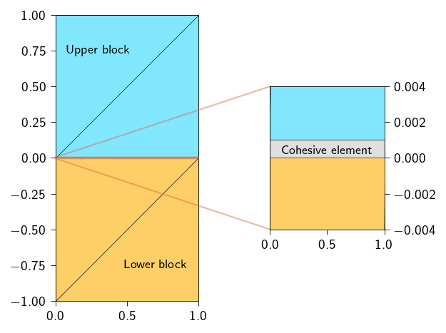
For understanding the cohesive zone approach, we will use a simple setting where fracture happens along a known plane. The setup comprises of two blocks of the same material. The fracture plane is the common interface between the two blocks. We use cohesive elements along this interface/plane to model the fracture or separation of the two blocks.

We discretize the two blocks using triangular elements. To keep things simple, we discretize each block into 2 elements. The two blocks are connected by cohesive element along the interface. Actually, the term cohesive element here is a misnomer, as we do not have any actual finite element along the interface. Rather, we use constraint technique to enforce how the two interfaces should separate. Since the constraints are applied to the displacements of nodes of the two interfaces of the blocks, we can think of the cohesive element as a 2D element with 4 nodes.

Note

For visualization purposes, we have separated the two 1D elements by a small \(\epsilon\). Ideally, the gap should be zero or extremely small (\(\approx 10^{-8}\) or \(10^{-10}\)).

eps = 1e-3
coords = np.array(
    [[0, -1], [1, -1], [1, 0], [0, 0], [0, eps], [1, eps], [1, 1], [0, 1]]
)

lower_elements = np.array([[0, 1, 2], [2, 3, 0]])
upper_elements = np.array([[4, 5, 6], [6, 7, 4]])

upper_elements_1d = np.array([[4, 5]])
lower_elements_1d = np.array([[2, 3]])

elements = np.vstack((upper_elements, lower_elements))

mesh = Mesh(coords, elements)


n_nodes = mesh.coords.shape[0]
n_dofs_per_node = 2
n_dofs = n_dofs_per_node * n_nodes

Code: Plot the mesh

plt.style.use(STYLE_PATH)
plt.figure(figsize=(6, 3), constrained_layout=True)
ax = plt.axes()

cb = ax.tripcolor(
    coords[:, 0],
    coords[:, 1],
    elements,
    facecolors=np.array([0, 0, 1, 1]),
    cmap="managua_r",
    shading="flat",
    edgecolors="black",
)


rect = plt.Rectangle((0, 0), 1, eps, color="grey", alpha=0.25)
ax.add_patch(rect)

x1, x2, y1, y2 = 0, 1, -0.004, 0.004  # subregion of the original image
axins = ax.inset_axes([1.5, 0.25, 0.8, 0.5], xlim=(x1, x2), ylim=(y1, y2))
axins.tripcolor(
    coords[:, 0],
    coords[:, 1],
    elements,
    facecolors=np.array([0, 0, 1, 1]),
    cmap="managua_r",
    shading="flat",
    edgecolors="black",
)
rect2 = plt.Rectangle((0, 0), 1, eps, color="grey", alpha=0.25)
axins.add_patch(rect2)
axins.yaxis.set_label_position("right")
axins.yaxis.tick_right()

ax.indicate_inset_zoom(axins, edgecolor=colors.red)
ax.set_xlim(0, 1)
ax.set_ylim(-1, 1)
ax.text(0.3, 0.75, "Upper block", ha="center", va="center", fontsize=8)
ax.text(0.7, -0.75, "Lower block", ha="center", va="center", fontsize=8)
ax.text(
    1.9, 50 * eps, "Cohesive element", ha="center", va="center", fontsize=8, zorder=20
)
ax.set_aspect("equal")

plt.show()

Figure 16.1: Code: Function to plot two blocks with fracture interface modelled using cohesive approach.

Defining material parameters

Let us define the material parameters mainly the shear modulus and the first Lamé parameter. The Youngs modulus and the Poisson’s ratio are related for the material are:

\[ E = 100.0 ~\text{N/m}^2, \quad \nu = 0.35 \]

From the above, we can compute the shear modulus and the first Lamé parameter as:

\[ \mu = \frac{E}{2(1+\nu)}, \quad \lambda = \frac{E\nu}{(1+\nu)(1-2\nu)} \]

class Material(NamedTuple):
    """Material properties for the elasticity operator."""

    mu: float  # Diffusion coefficient
    lmbda: float  # Diffusion coefficient

nu = 0.35

E = 100.0  # N/m^2
lmbda = nu * E / ((1 + nu) * (1 - 2 * nu))
mu = E / (2 * (1 + nu))



mat = Material(mu=mu, lmbda=lmbda)

Defining total elastic energy of the system

The total elastic energy of the system is given by:

\[ \Psi_\text{e}(\boldsymbol{u}) = \frac{1}{2} \int_\Omega \psi_e d\Omega \]

where

\[ \psi_\text{e}(x) = \boldsymbol{\sigma}(x) : \boldsymbol{\varepsilon}(x) \]

where \(\boldsymbol{\sigma}\) is the stress tensor and \(\boldsymbol{\varepsilon}\) is the strain tensor.

\[ \boldsymbol{\sigma} = \lambda \text{tr}(\boldsymbol{\varepsilon}) \mathbf{I} + 2\mu \boldsymbol{\varepsilon} \]

and

\[ \boldsymbol{\varepsilon} = \frac{1}{2} (\nabla \boldsymbol{u} + \nabla \boldsymbol{u}^T) \]

tri = element.Tri3()
op = Operator(mesh, tri)

# --- Material model (linear elasticity: plane strain) ---
@autovmap(grad_u=2)
def compute_strain(grad_u):
    return 0.5 * (grad_u + grad_u.T)

@autovmap(eps=2, mu=0, lmbda=0)
def compute_stress(eps, mu, lmbda):
    I = jnp.eye(2)
    return 2 * mu * eps + lmbda * jnp.trace(eps) * I

@autovmap(grad_u=2, mu=0, lmbda=0)
def strain_energy(grad_u, mu, lmbda):
    eps = compute_strain(grad_u)
    sigma = compute_stress(eps, mu, lmbda)
    return 0.5 * jnp.einsum("ij,ij->", sigma, eps)


@jax.jit
def total_strain_energy(u_flat: Array) -> float:
    """Compute the total energy of the system."""
    u = u_flat.reshape(-1, n_dofs_per_node)
    u_grad = op.grad(u)
    energy_density = strain_energy(u_grad, mat.mu, mat.lmbda)
    return op.integrate(energy_density)

Defining the fracture energy

Now let us define the fracture energy whcih is given by:

\[ \Psi_\text{fracture} = \int_{\Gamma_{coh}} \psi(\delta(\![\boldsymbol{u}]\!])) \text{d}a \]

In order to define the fracture energy, we need two things:

the traction-separation potential \(\psi(\delta(\![\boldsymbol{u}]\!]))\)
a way to integrate the traction-separation potential over the cohesive zone \(\Gamma_\text{coh}\)

Defining the operator for line integration

We will begin by defining the operator for line integration similar to Operator that we have used for the triangular elements. To do so, we will have to first define the line elements along the potential fracture surface. We will use the Line2 element to define the line elements. This element has 2 nodes. Below, we use the function extract_interface_mesh to generate the mesh that consists of the line elements along the potential fracture surface. Since are two blocks have two surfaces along which the fracture can propagate (upper and lower), we can use any one of the two surfaces to define the cohesive zone. Here, we use the lower surface. We will define a new mesh that contains the line elements from one of the two interfaces. Since the two interfaces are discretized using the same number of elements, and occupy the same spatial domain, we can use any one of the two to perform the integration.

def extract_interface_mesh(mesh, line_elements):
    """Generate a mesh for the interface between two materials."""
    
    # --- Interface mesh ---
    line_element_nodes = jnp.unique(line_elements.flatten())
    interface_coords = mesh.coords[line_element_nodes]
    interface_elements = jnp.array([[index, index + 1] for index in range(len(line_elements))])

    interface_mesh = Mesh(interface_coords, interface_elements)
    return interface_mesh

interface_mesh = extract_interface_mesh(mesh, lower_elements_1d)
line = element.Line2()
line_op = Operator(interface_mesh, line)

We will use the line_op to integrate the traction-separation potential \(\psi(\delta)\) over the cohesive zone \(\Gamma_\text{coh}\).

Defining the Traction-Separation potential

In order to define the traction-separation potential, we need

the critical stress \(\sigma_c\)
the fracture energy \(\Gamma\)
the penalty parameter \(\kappa\)
and a functional form of the traction-separation potential \(\psi(\delta)\)

Gamma = 5e-1  # J/m^2
sigma_c = 1.  # N/m^2

penalty = 1e8

Below define the functional form of the traction-separation potential \(\psi(\delta)\) for an exponential traction-separation law. The \(\psi(\delta)\) for an exponential traction-separation law is given by:

\[ \psi(\delta) = \begin{cases} \Gamma \left(1 - \left(1 + \frac{\delta}{\delta_c}\right) e^{-\frac{\delta}{\delta_c}}\right) & \text{for}~ \delta \ge 0 \\ \frac{1}{2} \kappa \delta^2 & \text{for}~ \delta < 0 \end{cases} \]

where \(\delta_c = \frac{\Gamma e^{-1}}{\sigma_c}\) is the critical separation, \(\Gamma\) is the fracture energy, \(\sigma_c\) is the critical stress, and \(e\) is the base of the natural logarithm.

Note

If you notice, the potential is also defined for \(\delta < 0\). When \(\delta < 0\), it means that the two surfaces are actually penetrating each other. In this case, we use a penalty like term to penalize the interpenetration. This is exactly similar to the penalty method used in the contact mechanics.

Remember at this point we do not introduce the irreversibility in the cohesive potential. This will be done in the next lectures.

In order to compute the \(\psi(\delta)\) for an exponential traction-separation law we need to perform the following steps:

Compute the opening \(\delta\) along the cohesive interface is defined as:

\[ \delta = \sqrt{ ([\![\boldsymbol{u}]\!] \cdot{}\boldsymbol{t})^2 + ([\![\boldsymbol{u}]\!] \cdot \boldsymbol{n})^2 } \]

where \(\boldsymbol{t}\) is the tangential direction (which for this problem is the \(x\)-direction) and \(\boldsymbol{n}\) is the normal direction to the cohesive interface (which for this problem is the \(y\)-direction).
Compute the cohesive energy density \(\psi(\delta)\) using the exponential traction-separation potential.

\[ \psi(\delta) = \psi(\delta(\![\boldsymbol{u}]\!])) \]

Hint

The function to compute the opening of the cohesive element will look like this:

@autovmap(jump=1)
def compute_opening(jump: jnp.ndarray) -> float:
    """
    Compute the opening of the cohesive element.
    Args:
        jump: The jump in the displacement field, which is the difference between the displacement of the upper and lower bodies across the crack.
    Returns:
        The opening of the cohesive element.
    """
    opening = ... # TODO: Compute the opening of the cohesive element
    return opening

The function to compute the cohesive energy density will look like this:

@autovmap(jump=1)
def exponential_cohesive_energy(
    jump: jnp.ndarray,
    Gamma: float,
    sigma_c: float,
    penalty: float,
    delta_threshold: float = 0.0,
) -> float:
    """
    Compute the cohesive energy for a given jump. 
    Args:
        jump: The jump in the displacement field.
        Gamma: Fracture energy of the material.
        sigma_c: The critical strength of the material.
        penalty: The penalty parameter for penalizing the interpenetration.
    """

    delta = ... # TODO: Compute the opening of the cohesive element

    ... # TODO: check if delta is greater than the threshold

    ... # TODO: if delta is greater than the threshold, compute the cohesive energy density using the exponential traction-separation potential

    ... # TODO: if delta is less than the threshold, return 0.5 * penalty * delta**2

    return cohesive_energy_density

In order to check if the delta is greater than the threshold, use the jax.lax.cond function.

Moreover, use the below defined safe_sqrt function to compute the square root of the delta. We redefine the square root function because default square root function is non-differentiable at zero because of the limit definition of the square root. Here we use the jnp.where function to return zero when the input is less than or equal to zero. This makes the square root function differentiable at zero.

@jax.jit
def safe_sqrt(x):
    return jnp.sqrt(jnp.where(x > 0., x, 0.))

@jax.jit
def safe_sqrt(x):
    return jnp.sqrt(jnp.where(x > 0., x, 0.))


@autovmap(jump=1)
def compute_opening(jump: jnp.ndarray) -> float:
    """
    Compute the opening of the cohesive element.
    Args:
        jump: The jump in the displacement field.
    Returns:
        The opening of the cohesive element.
    """
    opening = safe_sqrt(jump[0] ** 2 + jump[1] ** 2)

    return opening


@autovmap(jump=1)
def exponential_cohesive_energy(
    jump: jnp.ndarray,
    Gamma: float,
    sigma_c: float,
    penalty: float,
    delta_threshold: float = 0.0,
) -> float:
    """
    Compute the cohesive energy for a given jump. 
    Args:
        jump: The jump in the displacement field.
        Gamma: Fracture energy of the material.
        sigma_c: The critical strength of the material.
        penalty: The penalty parameter for penalizing the interpenetration.
        delta_threshold: The threshold for the delta parameter.
    Returns:
        The cohesive energy.
    """
    delta = compute_opening(jump)
    delta_c = (Gamma * jnp.exp(-1)) / sigma_c

    def true_fun(delta):
        return Gamma * (1 - (1 + (delta / delta_c)) * (jnp.exp(-delta / delta_c)))

    def false_fun(delta):
        return 0.5 * penalty * delta**2

    return jax.lax.cond(delta > delta_threshold, true_fun, false_fun, delta)


cohesive_traction = jax.jacrev(exponential_cohesive_energy)
cohesive_stiffness = jax.jacfwd(cohesive_traction)

Now we can use the line_op to integrate the traction-separation potential \(\psi(\delta)\) over the cohesive zone \(\Gamma_\text{coh}\).

\[ \Psi_\text{fracture} = \int_{\Gamma_{coh}} \psi(\delta) \text{d}a \]

We will need the nodes associated with the interface elements to later compute the jump between the lower and upper bodies across the crack.

lower_cohesive_nodes = jnp.unique(lower_elements_1d.flatten())
upper_cohesive_nodes = jnp.unique(upper_elements_1d.flatten())
print(lower_cohesive_nodes)
print(upper_cohesive_nodes)

[2 3]
[4 5]

Note

The function to compute the cohesive energy will look like this:

def total_fracture_energy(u_flat: Array, upper_cohesive_nodes: Array, lower_cohesive_nodes: Array) -> float:
    """
    Compute the total fracture energy of the system.
    Args:
        u_flat: The flat displacement vector
        upper_cohesive_nodes: The nodes associated with the upper cohesive surface.
        lower_cohesive_nodes: The nodes associated with the lower cohesive surface.
    Returns:
        The total cohesive energy of the system.

    """
    # TODO: reshape the flat displacement vector to the displacement field
    u = ... 
    
    # TODO: compute the jump in the displacement field between the upper and lower bodies across the crack, 
    # make use of the `upper_cohesive_nodes` and `lower_cohesive_nodes`
    jump = ... 

    # TODO: evaluate the jump at the quad points using the `line_op.eval` function
    jump_quad = ... 
    
    # TODO: compute the cohesive energy density using the `exponential_cohesive_energy` function
    cohesive_energy_density = ... 
    
    # TODO: integrate the cohesive energy density over the cohesive zone using the `line_op.integrate` function
    cohesive_energy = ... 
    
    return cohesive_energy


@jax.jit
def total_cohesive_energy(u_flat: Array) -> float:
    u = u_flat.reshape(-1, n_dofs_per_node)
    jump = u.at[upper_cohesive_nodes, :].get() - u.at[lower_cohesive_nodes, :].get()
    jump_quad = line_op.eval(jump)
    cohesive_energy_density = exponential_cohesive_energy(
        jump_quad, Gamma, sigma_c, penalty
    )
    return line_op.integrate(cohesive_energy_density)

Defining the total potential energy

\[ \Psi = \Psi_\text{elastic} + \Psi_\text{fracture} \]

@jax.jit
def total_energy(u_flat: jnp.ndarray) -> float:
    u = u_flat.reshape(-1, n_dofs_per_node)
    elastic_strain_energy = total_strain_energy(u)

    cohesive_energy = total_cohesive_energy(u)
    return elastic_strain_energy + cohesive_energy

How is cohesive approach similar to Penalty constrained approach?

As we mentioned in the last chapter, the cohesive approach is similar to the penalty constrained approach. This is because we are tying two surfaces together using a penalty like parameter. The only difference is that in the cohesive approach, we are using a traction-separation potential to tie the two surfaces together, while in the penalty constrained approach, we are using a penalty function.

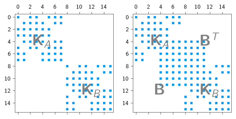
We can actually see that the cohesive approach is similar to the penalty constrained approach by plotting the stiffness matrix of the above problem. Below we plot the stiffness matrix of the cohesive approach for the case when we do not consider the cohesive zone and when we consider the cohesive zone. As we can see the stiffness matrix without the cohesive zone is a block diagonal matrix with the two blocks corresponding to the upper and lower blocks.

\[ \mathbf{K} = \begin{bmatrix} \mathbf{K}_\text{upper} & 0 \\ 0 & \mathbf{K}_\text{lower} \end{bmatrix} \]

The stiffness matrix with the cohesive zone is a block diagonal matrix with the two blocks corresponding to the upper and lower blocks and the cohesive zone and the two blocks are connected by the cohesive zone.

\[ \mathbf{K} = \begin{bmatrix} \mathbf{K}_\text{upper} & \mathbf{K}_\text{cohesive}^{T} \\ \mathbf{K}_\text{cohesive} & \mathbf{K}_\text{lower} \end{bmatrix} \]

which is similar to the stiffness matrix of the penalty constrained approach (In-class activity: Node-to-Surface Contact)

\[ \mathbf{K} = \begin{bmatrix} \mathbf{K}_{A} & \mathbf{B}^{T} \\ \mathbf{B} & \mathbf{K}_{B} \end{bmatrix} \]

Stiffness matrix of the cohesive approach. The stiffness matrix on the left is when we do not consider the cohesive zone, while the stiffness matrix on the right is when we consider the cohesive zone.

Let us now break the two blocks

We now break the two blocks along the interface. To this end, we apply a displacement to the upper block along the interface. We will apply a Mode I loading to the upper block.

\[ u_y(y=y_{max}) = 1.0, \quad u_x(y=y_{max}) = 0.0 \]

We keep the lower part of the lower block fixed in both the \(x-\) and \(y-\) directions. \[ u_x(y=y_{min}) = 0.0, \quad u_y(y=y_{min}) = 0.0 \]

Code

y_min = np.min(coords[:, 1])
y_max = np.max(coords[:, 1])
fixed_nodes = np.where(jnp.isclose(coords[:, 1], y_min))[0]
loaded_nodes = np.where(jnp.isclose(coords[:, 1], y_max))[0]

# --- Apply Dirichlet BCs ---
fixed_dofs = jnp.concatenate(
    [
        2 * fixed_nodes,
        2 * fixed_nodes + 1,
        2 * loaded_nodes,
        2 * loaded_nodes + 1,
    ]
)


all_dofs = jnp.arange(n_dofs)
free_dofs = jnp.setdiff1d(all_dofs, fixed_dofs)


prescribed_values = jnp.zeros(n_dofs)
prescribed_values = prescribed_values.at[2 * loaded_nodes + 1].set(1.0)

Using matrix-free solver

Now, we define a few functions to implement the matrix-free solvers. We will use the conjugate gradient method to solve the linear system of equations. The Dirichlet boundary conditions are applied using projection method. As we use the matrix-free solver, we need to define the gradient of the total potential energy, which is also the residual function.

\[ \boldsymbol{r} = \boldsymbol{f}_{ext} - \boldsymbol{f}_{int} \]

where \(\boldsymbol{f}_{ext}\) is the external force vector and \(\boldsymbol{f}_{int}\) is the internal force vector given by the gradient of the total potential energy.

\[ \boldsymbol{f}_{int} = \frac{\partial \Psi}{\partial \boldsymbol{u}} \]

We also define a function to compute the JVP product to compute the incremental residual for an increment in the displacement.

\[ \delta \boldsymbol{f}_{int} = \frac{\partial \boldsymbol{f}_{int}}{\partial \boldsymbol{u}}|_{\boldsymbol{u}=\boldsymbol{u}_\mathrm{prev}} \delta \boldsymbol{u} \]

Below, we define the functions to compute the gradient and the Jacobian-vector product (JVP). Within the Jacoboian-Vector product, we apply Projection approach by first “zeroing” out the displacements and then “zeroing” out the residual at the fixed DOFs. See Matrix-free solvers and In-class activity: Node-to-Surface Contact for more details on how to compute the Jacobian-vector product using jax.jvp.

Hint

Below define the function to compute the \(\boldsymbol{f}_{int}\) using jax.jacrev and then use this function to compute the Jacobian-vector product using jax.jvp. Remember to apply the Projection approach to enforce the Dirichlet boundary conditions.

# creating functions to compute the gradient and
gradient = jax.jacrev(total_energy)


# create a function to compute the JVP product
@jax.jit
def compute_tangent(du, u_prev):
    du_projected = du.at[fixed_dofs].set(0)
    tangent = jax.jvp(gradient, (u_prev,), (du_projected,))[1]
    tangent = tangent.at[fixed_dofs].set(0)
    return tangent

Below we define the Conjugate-gradient method and the Newton-Rahpson method to solve the nonlinear problem of contact. See Matrix-free solvers and In-class activity: Node-to-Surface Contact for more details on how to implement Conjugate-gradient and Newton-Raphson methods for matrix-free solvers.

Hint

We need to define two functions:

def conjugate_gradient(...):
    ...

def newton_krylov_solver(...):
    ...

Code: Functions to implement the conjugate gradient method and Netwon-Raphson method

from functools import partial
import equinox as eqx

#@partial(jax.jit, static_argnames=["A", "atol", "max_iter"])
@eqx.filter_jit
def conjugate_gradient(A, b, atol=1e-8, max_iter=100):

    iiter = 0

    def body_fun(state):
        b, p, r, rsold, x, iiter = state
        Ap = A(p)
        alpha = rsold / jnp.vdot(p, Ap)
        x = x + jnp.dot(alpha, p)
        r = r - jnp.dot(alpha, Ap)
        rsnew = jnp.vdot(r, r)
        p = r + (rsnew / rsold) * p
        rsold = rsnew
        iiter = iiter + 1
        return (b, p, r, rsold, x, iiter)

    def cond_fun(state):
        b, p, r, rsold, x, iiter = state
        return jnp.logical_and(jnp.sqrt(rsold) > atol, iiter < max_iter)

    x = jnp.full_like(b, fill_value=0.0)
    r = b - A(x)
    p = r
    rsold = jnp.vdot(r, p)

    b, p, r, rsold, x, iiter = jax.lax.while_loop(
        cond_fun, body_fun, (b, p, r, rsold, x, iiter)
    )
    return x, iiter


def newton_krylov_solver(
    u,
    fext,
    gradient,
    fixed_dofs,
):
    fint = gradient(u)

    du = jnp.zeros_like(u)

    iiter = 0
    norm_res = 1.0

    tol = 1e-8
    max_iter = 10

    while norm_res > tol and iiter < max_iter:
        residual = fext - fint
        residual = residual.at[fixed_dofs].set(0)
        A = eqx.Partial(compute_tangent, u_prev=u)
        du, cg_iiter = conjugate_gradient(A=A, b=residual, atol=1e-8, max_iter=100)

        u = u.at[:].add(du)
        fint = gradient(u)
        residual = fext - fint
        residual = residual.at[fixed_dofs].set(0)
        norm_res = jnp.linalg.norm(residual)
        print(f"  Residual: {norm_res:.2e}")
        iiter += 1

    return u, norm_res

Implementing the Incremental Loading Loop

Now that we have the mesh, the energy functions, and the newton_krylov_solver, it’s time to set up the main simulation loop. We will apply the displacement in small increments and solve for equilibrium at each step.

We divide the total displacement into 5 steps and solve the system of equations for each step.

Within each step, we will also store the applied displacement on the top surface and the reaction traction on the top surface. Later we will use this data to plot the traction-displacement curve.

Hint

The loop will look like this:

for step in range(n_steps):
    print(f"Step {step+1}/{n_steps}")
    # ... Your code for each step will go inside this loop ...

u_prev = jnp.zeros(n_dofs)
fext = jnp.zeros(n_dofs)

n_steps = 20

u_per_step = []

force_on_top = []
displacement_on_top = []

force_on_top.append(0)
displacement_on_top.append(0)

du_total = prescribed_values / n_steps  # displacement increment
for step in range(n_steps):
    print(f"Step {step+1}/{n_steps}")
    u_prev = u_prev.at[fixed_dofs].add(du_total[fixed_dofs])

    u_new, rnorm = newton_krylov_solver(
        u=u_prev,
        fext=fext,
        gradient=gradient,
        fixed_dofs=fixed_dofs,
    )

    u_prev = u_new
    force_on_top.append(jnp.sum(gradient(u_prev)[2 * loaded_nodes + 1]))
    displacement_on_top.append(jnp.mean(u_prev[2 *loaded_nodes + 1]))
    u_per_step.append(u_prev.reshape(n_nodes, n_dofs_per_node))

u_solution = u_prev.reshape(n_nodes, n_dofs_per_node)

Post-processing

Code: To generate deformed bodies and force-displacement curve

from matplotlib.gridspec import GridSpec

# squeeze to remove the quad point dimension (only 1 quad point)
grad_u = op.grad(u_solution).squeeze()
strains = compute_strain(grad_u)
stresses = compute_stress(strains, mat.mu, mat.lmbda)

delta_c  = (Gamma * jnp.exp(-1)) / sigma_c

fig = plt.figure(layout="constrained", figsize=(6, 2))

gs = GridSpec(1, 4, figure=fig, width_ratios=[0.2, 0.2, 0.2, 0.8], wspace=0.1)
ax = fig.add_subplot(gs[0, 0])
plot_nodal_values(
    u=u_per_step[1],
    mesh=mesh,
    nodal_values=u_per_step[1][:, 1].flatten(),
    ax=ax,
    label=r"$u_{y}$",
    shading="flat",
    edgecolors="black",
)
ax.margins(x=0, y=0)
ax.set_ylim(-1, 2)
ax.spines[['right', 'top']].set_visible(False)


ax = fig.add_subplot(gs[0, 1])
plot_nodal_values(
    u=u_per_step[5],
    mesh=mesh,
    nodal_values=u_per_step[5][:, 1].flatten(),
    ax=ax,
    label=r"$u_{y}$",
    shading="flat",
    edgecolors="black",
)
ax.margins(x=0, y=0)
ax.set_ylim(-1, 2)
ax.axis("off")

ax = fig.add_subplot(gs[0, 2])
plot_nodal_values(
    u=u_solution,
    mesh=mesh,
    nodal_values=u_solution[:, 1].flatten(),
    ax=ax,
    label=r"$u_y$",
    shading="flat",
    edgecolors="black",
)
ax.margins(x=0, y=0)
ax.set_ylim(-1, 2)
ax.axis("off")

ax = fig.add_subplot(gs[0, 3])
ax.plot(displacement_on_top, force_on_top, "o-")
ax.axvline(delta_c, color=colors.red, linestyle="--", label=r"$\delta_c$")
ax.axhline(sigma_c, color=colors.green, linestyle="--", label=r"$\sigma_c$")
ax.set_ylim(0, 1.1*sigma_c)
ax.text(1.2*delta_c, 0.5*sigma_c, r"$\delta_c$", color=colors.red, ha="center", va="center")
ax.text(0.5, 0.95*sigma_c, r"$\sigma_c$", color=colors.green, ha="center", va="center")
ax.margins(0, 0)
ax.set_xlabel("Displacement on top")
ax.set_ylabel("Traction on top")
ax.grid(True)
ax.ticklabel_format(axis="both", style="sci", scilimits=(1, -4))

plt.show()

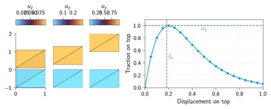
Snapshots of the deformed body at different stages of loading showing the decohesion process. The figure on the right shows how the traction on the top surface changes with the displacement on the top surface.