In this exercise, we will see an application of constraint handling in FEM and we will apply Dirichlet boundary conditions as constraints. The problem is the same as in the previous exercises.
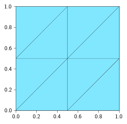
We have a unit square domain \(\Omega = [0, 1] \times [0, 1]\) which fixed in space in both \(x\) and \(y\) directions on the left edge. We apply a displacement along \(x-\)direction on the right edge. The applied displacement is \(0.3\). Furthermore, the domain is discretized using triangular elements.
The assumptions that we make in this exercise are:
linear elastic material
infinitesimal strains under plain strain conditions
In this exercise, we explore the constrained problem with:
equality constraint i.e\(g_i(u) = 0\)
active set is known and does not change i.e we always know which degrees of freedom are in \(\mathcal{A}\)
The objective of this exercise is to use the Lagrange multiplier method to enforce the Dirichlet boundary conditions. We will use the Lagrange multiplier method to enforce the Dirichlet boundary conditions on the right edge as well as the left edge of the domain. Later, we will see how exact the constraints are enforced..
Below is the expected workflow for solving this exercise.
Workflow
As we have mentioned, our way of solving any problem in this course is to define a python function that computes the total potential energy \(\Psi\).
For this specific problem, instead of the total potential energy, we will define the Lagrangian functional \(\mathcal{L}\) which is given as
Similar to previous exercises, we consider a unit square domain \(\Omega = [0, 1] \times [0, 1]\) which fixed in space in both \(x\) and \(y\) directions on the right edge. We apply a displacement along \(x-\)direction on the left edge. Furthermore, the domain is discretized using triangular elements.
Let us define the material parameters mainly the shear modulus and the first Lamé parameter.
\[
\mu = 0.5, \quad \lambda = 1.0
\]
class Material(NamedTuple):"""Material properties for the elasticity operator.""" mu: float# Shear modulus lmbda: float# First Lamé parametermat = Material(mu=0.5, lmbda=1.0)
Defining the total elastic energy
We would now define a function that computes the total energy of the system.
\[
\epsilon = \frac{1}{2} (\nabla u + \nabla u^T)
\]
Hint
To do so, we must perform the following steps:
Define the triangular element from tatva.element.
Define the Operator object from tatva.operator which takes the mesh and the element as input.
Define the function that computes the total energy by performing following operations:
Compute the gradient of the displacement, uses Operator.grad.
Compute the strain energy density, use the function defined above
Integrate the strain energy density over the domain, use Operator.integrate.
Code: Defining the material properties and the strain energy density
tri = element.Tri3()op = Operator(mesh, tri)@autovmap(grad_u=2)def compute_strain(grad_u: Array) -> Array:"""Compute the strain tensor from the gradient of the displacement."""return0.5* (grad_u + grad_u.T)@autovmap(eps=2, mu=0, lmbda=0)def compute_stress(eps: Array, mu: float, lmbda: float) -> Array:"""Compute the stress tensor from the strain tensor.""" I = jnp.eye(2)return2* mu * eps + lmbda * jnp.trace(eps) * I@autovmap(grad_u=2, mu=0, lmbda=0)def strain_energy(grad_u: Array, mu: float, lmbda: float) -> Array:"""Compute the strain energy density.""" eps = compute_strain(grad_u) sig = compute_stress(eps, mat.mu, mat.lmbda)return0.5* jnp.einsum("ij,ij->", sig, eps)@jax.jitdef total_elastic_energy(u_flat: Array) ->float:"""Compute the total energy of the system.""" u = u_flat.reshape(-1, n_dofs_per_node) u_grad = op.grad(u) energy_density = strain_energy(u_grad, mat.mu, mat.lmbda)return op.integrate(energy_density)
Defining Dirichlet boundary conditions as constraints
We now define the degrees of freedom that for the left edge of the domain and the right edge of the domain. These are the degrees of freedom that are associated with the nodes on the left and right edge of the domain.
Remember that on the left edge, we have both \(x\) and \(y\) degrees of freedom fixed (\(u_x=u_y=0\)) and on the right edge, we have apply a displacement of 0.3 on \(x\) degree of freedom (\(u_x=0.3\)).
Hint
It might be best to store all the degrees of freedom where displacement is applied (either 0 or 0.3) as vector named constrained_dofs.
We now define a constraints that enforces the Dirichlet boundary conditions on the degrees of freedom associated with the nodes on the right edge of the domain. Let us denote the applied displacement as \(u_d\). The constraint then is defined as
\[
u_x^{i} = u_d \quad \forall i \in \mathcal{A}
\]
where \(\mathcal{A}\) is the set of degree of freedoms associated with the nodes on the right edge of the domain. We will refer to \(\mathcal{A}\) as active set.
We can define the constraint as a function of the degrees of freedom as follows:
\[
g_i(u) = u_{x}^{i} - u_d
\]
Hint
The function definition will be something like this:
def equality_constraints(u, constraints):"""Compute the constraint vector g(u) Args: u: the displacement vector, a vector of size n_dofs constraints: the applied displacement at the constrained_dofs, a vector of size nb_cons Returns: the constraint vector of size equal to the nb_cons """# get the displacement values at constrained dofs from u ...# compute the g(u) i.e. difference between the above displacement values and the applied displacement ...# return the constraint vectorreturn ...
The Lagrange functional is defined as \[
\mathcal{L}(\boldsymbol{u}, \boldsymbol{\lambda}) = \Psi_\text{e}(\boldsymbol{u}) + \boldsymbol{\lambda}\cdot{} g(\boldsymbol{u})
\]
where \(\mathcal{A}\) is the set of degrees of freedom associated with the nodes on the right edge and the left edge of the domain. Notice that there is no condition on \(\lambda\) unlike the KKT condition for the inequality constraints. This is because depending on how the constraint \(g_i(u)\) is violated, the \(\lambda\) will adapt its nature (i.e sign of the constraining force to meet the equality constraint).
Write a function that computes the lagrange functional as defined above. We will define a vector \(\boldsymbol{z}\) which is the concatenation of the displacement vector \(\boldsymbol{u}\) and the Lagrange multiplier vector \(\boldsymbol{\lambda}\).
The function should take the vector \(\boldsymbol{z}\) and a constraints vector that needs to be enforced as input and return the value of the Lagrangian functional.
Hint
The function definition will be something like this:
def lagrange_functional(z, constraints):"""Compute the lagrange functional Args: z: the vector of degrees of freedom and lagrange , a vector of size (n_dofs + nb_cons) constraints: the applied displacement, a vector of size (nb_cons) Returns: the value of the lagrange functional, a scalar """ u = z.at[:-nb_cons].get() # we get the displacement vector from the vector z _lambda = z.at[-nb_cons:].get() # we get the lagrange multiplier vector from the vector z# use u to compute the elastic energy ...# use u, _lambda and above defined equality constraint to compute the energy due to lagrange multiplier ...# add the two energies ...# return the total energyreturn ...
We will also need the derivative of the above defined Lagrange functional and the second derivative of it. \[
\frac{\partial \mathcal{L}}{\partial z}, \quad \frac{\partial^2 \mathcal{L}}{\partial z^2}
\]
For this part of the exercise, we will compute a dense stiffness matrix \(\frac{\partial^2 \mathcal{L}}{\partial z^2}\). Later in the exercise, we will compute a sparse stiffness matrix.
Hint
Use JAX to differentiate the above defined function lagrange_functional. Be careful with the use of jax.jacrev and jax.jacfwd.
dLdz = # to define the function to compute derivative of `lagrange_functional`
d2Ldz2 = # to define the function to compute the derivative of `dLdz` which will be the dense stiffness matrix
As we mentioned to solve a saddle-point problem, the best way is to use a direct linear solver. We will use the jnp.linalg.solve function to solve the linear system. Below, we define a newton solver that uses direct linear solver.
Remember here we solve the dense stiffness matrix and later we will solve the sparse stiffness matrix.
Hint
We no longer need lifting approach to enforce the boundary conditions. This is taken care by the constraint enforcement through lagrange multiplier approach. So do not perform the lifting of the stiffness matrix and the residual vector.
In order to solve the above linear system, you will need to define a newton_solver function. Remember this will use a dense stiffness matrix therefore we cannot use the newton_sparse_solver function from the penalty method exercise.
The function definition will be something like this:
def newton_solver(z, gradient, hessian, constraints, ...):"""Newton solver to solve the linear system Args: z: the vector of degrees of freedom and lagrange multiplier, a vector of size (n_dofs + nb_cons) gradient: a function that computes the gradient of the lagrange functional hessian: a function that computes the dense hessian of the lagrange functional constraints: the applied displacement, a vector of size (nb_cons) ...: other arguments if needed Returns: the solution vector, a vector of size (n_dofs + nb_cons) and the norm of the residual, a scalar """# compute the internal force vector ...# check if norm of the residual is less than the tolerance or the number of iterations is greater than the maximum number of iterations ...# start the while loopwhile ...:# compute the residual vector ...# compute the dense stiffness matrix, since it is dense we will not use the sparse solver ...# solve the linear system ...# update the solution ...# compute the residual ...# check if the residual is less than the tolerance ...# return the solution and the norm of the residualreturn ...
def newton_solver(z, gradient, hessian, linear_solver=jnp.linalg.solve): iiter =0 norm_res =1.0 tol =1e-8 max_iter =10while norm_res > tol and iiter < max_iter: residual =-gradient(z) K = hessian(z) dz = linear_solver(K, residual) z = z.at[:].add(dz) residual =-gradient(z) norm_res = jnp.linalg.norm(residual)print(f" Residual: {norm_res:.2e}") iiter +=1return z, norm_res
Now, lets us solve the problem using the above defined newton solver to find the solution. We solve the problem in 10 steps.
We now check how well the lagrange multiplier is able to enforce the constraints. We do this by checking the value of the displacement at the right edge of the domain and the left edge of the domain.
The displacement (in \(x-\)direction) at the right edge of the domain should be \(0.3\)i.e.
\[
u_x = 0.3
\]
and the displacement at the left edge of the domain should be \(0\)i.e.
\[
u_x = 0
\]
Please implement the above checks and print the values of the displacements at the right and left edges of the domain and see how close they are to the exact values.
u_solution.at[right_nodes, 0].get()
Array([0.3, 0.3, 0.3], dtype=float64)
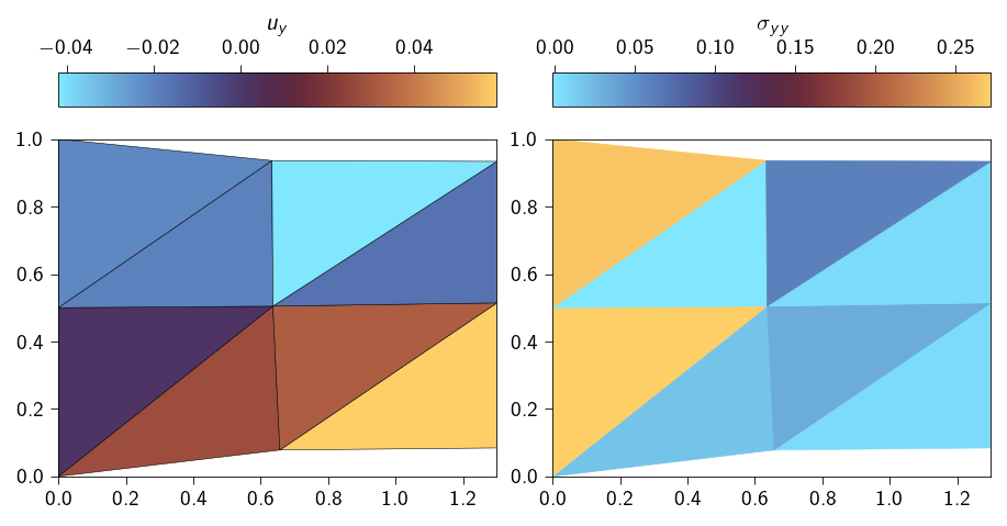
Lets plot to the deformed shape of the domain to see if the constraints are met.
Code: Plotting the solution from direct linear solver
As we mentioned in the previous section, \(\lambda\), the lagrange multiplier, is the force applied to the system to enforce the constraint.
What is the nature of the force applied? Is it pulling the body to meet the constraint (hence positive) or is it squeezing the body to meet the constraint (hence negative).
Compute the internal force vector and compare it with the Lagrange multiplier vector. Are both equal?
If you compare the solution for this problem with Penalty method, how exact or inexact the constraints are met?
Sparse solver
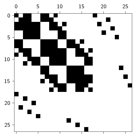
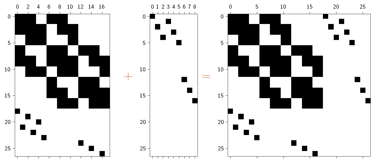
If we look at the full stiffness matrix, we can see that it is a sparse matrix. As we have seen in the previous section, the sparsity pattern of the KKT system is the union of the sparsity patterns of the matrices \(\mathbf{K}\) and \(\mathbf{B}\). We can use this property to construct the sparsity pattern for the KKT system.
To use the direct sparse solver, we need to convert the KKT system into a sparse format. Similar to the exercise in Sparse solvers, we will need to define the sparsity pattern for the KKT system. If we look at the full KKT system as shown below,
we can see that the sparsity pattern of the KKT system is the union of the sparsity patterns of the matrices \(\mathbf{K}\) and \(\mathbf{B}\). From the previous section Sparse solvers, we know how to construct the sparsity pattern for the matrix \(\mathbf{K}\).
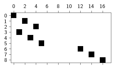
We can use the jax.jacrev function to automatically compute the Jacobian of the equality_constraints function. Remember that \(\mathbf{B}\) is given as
where \(\mathbf{g}\) is the constraint function. We will use this property of \(\mathbf{B}\) to compute it automatically. This could be useful for cases where the constraint function is complex and difficult to compute manually.
B = jax.jacrev(equality_constraints)(jnp.zeros(n_dofs), constraints).astype(jnp.int32)
In the figure below we show the sparsity pattern for the matrix \(\mathbf{B}\).
Code: Plotting the sparsity pattern for the matrix \(\mathbf{B}\)
We construct the sparsity pattern for the KKT system in two parts. First, we construct the sparsity pattern for the left-hand side of the KKT system. This is the sparsity pattern for the matrix \(\mathbf{K}\) and \(\mathbf{B}\). We then construct the sparsity pattern for the right-hand side of the KKT system. This is the sparsity pattern for the matrix \(\mathbf{B}^T\) and \(\mathbf{0}\). We then concatenate the two sparsity patterns to get the sparsity pattern for the full KKT system.
Step-by-step construction of the sparsity pattern for the KKT system
We provide the functionality to create the sparsity pattern for the KKT system in the sparse module. To do this we need to pass the mesh, the number of degrees of freedom per node and the matrix \(\mathbf{B}\) to the sparse.create_sparsity_pattern_KKT function. Behind the scenes, the function will compute the sparsity pattern for the matrix \(\mathbf{K}\) and \(\mathbf{B}\) and then concatenate them to get the sparsity pattern for the full KKT system as we have done above.
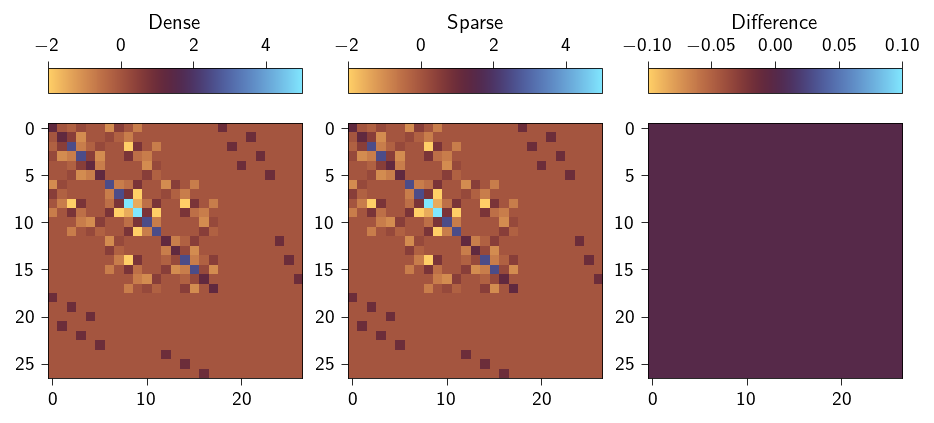
Now, lets us verify that the generated sparsity pattern is correct or not. To do so, we will derive the KKT system first, directly differentiating the functional \(\partial \mathcal{L}/\partial \boldsymbol{z}\) with respect to the degrees of freedom and the Lagrange multipliers. Then, we will do the same but by sparsely differentiating the \(\partial \mathcal{L}/\partial \boldsymbol{z}\) with respect to the degrees of freedom and the Lagrange multipliers. To do this we will use the sparse.jacfwd with the above defined sparsity pattern.
We now plot the full KKT matrix K_dense as derived in the dense format and the sparse matrix K_sparse from sparse differentiation. Below, we also show the difference between the two matrices.
Comparison of the KKT matrix in dense and sparse format
Now we will use the above defined sparse stiffness matrix K_sparse to solve the KKT system.
We define a newton solver that uses a sparse linear solver. We use the sparse solver from scipy.sparse.linalg.spsolve. Note that we need to convert the sparse matrix to a CSR matrix before passing it to the sparse solver.
Hint
We no longer need lifting approach to enforce the boundary conditions. This is taken care by the constraint enforcement through lagrange multiplier approach. So do not perform the lifting of the stiffness matrix and the residual vector.
You can use the newton_sparse_solver function from the penalty method exercise.
import scipy.sparse as spdef newton_sparse_solver(z, gradient, hessian, linear_solver=sp.linalg.spsolve):""" Newton solver with sparse linear solver. """ iiter =0 norm_res =1.0 tol =1e-8 max_iter =10while norm_res > tol and iiter < max_iter: residual =-gradient(z) K_sparse = hessian(z) K_csr = sp.csr_matrix( (K_sparse.data, (K_sparse.indices[:, 0], K_sparse.indices[:, 1])) ) dz = linear_solver(K_csr, residual) z = z.at[:].add(dz) residual =-gradient(z) norm_res = jnp.linalg.norm(residual)print(f" Residual: {norm_res:.2e}") iiter +=1return z, norm_res
Let us now solve the problem with the sparse solver.