In this exercise, we will solve numerically the problem of contact between two elastic bodies. Unlike the last exercise, where we studied the contact between a deformable body and a rigid body, here we need to detect which part of the two bodies are coming in contact. Therefore, in order to correctly account for the contact between the bodies we will first, implement a contact detection algorithm to capture which part of the upper surface comes in contact with the lower body and then use the gap function to compute the contact energy using the Penalty method.
An animation of the contact between two elastic bodies is shown below.
Therefore, for this in-class activity we have two objectives:
Implement a contact detection algorithm. In this activity, we will use the node-to-surface approach to compute the above gap function (see Fundamentals).
Use the contact detection algorithm to formulate the contact energy using penalty method.
Similar to last exercise, we will use the normal gap function between the surfaces of the two bodies to determine when the two bodies come in contact
Doing node-to-surface detection means we have to perform the following steps for each node on the contactor surface:
Construct the outward normal \(\boldsymbol{n}\)of every element on the opposing target surface.
Calculate the projection point \(\boldsymbol\rho\)of every element on the opposing target surface.
Calculate the distance between the contactor node and the projection point for every element on the opposing target surface.
Filter the results to find the best valid point, the corresponding target element, and the normal at the contact point.
Calculate the normal gap.
Step 1: Find the outward normal
Implement a function that returns the outward normal vector for one element of the target surface. Use @autovmap to automatically vectorize the function for an array of line segments.
Hint
The function implement will look something like this:
@autovmap(surface_points=2, reference_point=1)def find_normal_to_surface(surface_points : Array, reference_point : Array) -> Array:""" Find the normal to the surface at a point. Args: surface points: Coordinates of the target surface element, shape (2, 2) reference_point: Coordinates of a known reference point which is inside the surface/body, shape (2,) Returns: normal: The outward normal to the surface, shape (2,) """# TODO: Implement the functionreturn ...
Use jnp.linalg.norm to normalize the normal vector,jnp.vdot to compute the dot product and jnp.where to flip the sign of the normal vector if it points away from the reference point.
Code: Find the outward normal to a surface
@autovmap(surface_points=2, reference_point=1)def find_normal_to_surface(surface_points: Array, reference_point: Array) -> Array:""" Find the normal to the surface at a point. Args: surface_points: The coordinates of the surface points. reference_point: The coordinates of the reference point which is inside the surface. Returns: normal: The normal to the surface at the reference point. """ tangent_vector = surface_points[1] - surface_points[0] normal = jnp.array([-tangent_vector[1], tangent_vector[0]]) normal = normal / jnp.linalg.norm(normal) reference_vector = reference_point - surface_points[0] normal_sign = jnp.vdot(reference_vector, normal) normal = jnp.where(normal_sign >0, -normal, normal)return normal
Step 2: Calculate the projection point
Implement a function that returns the projection point \(\boldsymbol\rho\) for one contactor-point/target-surface-element pair.
Hints
The function implementation will be something like this:
@autovmap(point=1, surface_coords=2, surface_normal=1)def find_projection_point():""" Find the projection point to a plane from a point. Args: point: The contactor point to find the orthogonal point to, shape (2,) surface_coords: The points on the surface, shape (2, 2) surface_normal: The outward normal to the surface element, shape (2,) Returns: projection_point: The projection point to the surface, shape (2,) """return ...
@autovmap(point=1, surface_coords=2, surface_normal=1)def find_projection_point( point: Array, surface_coords: Array, surface_normal: Array) ->float:""" Find the orthogonal point to a plane from a point. """ numerator = jnp.vdot(point - surface_coords[0], surface_normal) normal = jnp.linalg.norm(surface_normal) projection_point = point - numerator * surface_normal / normal**2return projection_point
Step 3: Calculate Distance and Check Bounds
In this function, we will perform two critical operations:
Check if the projection from find_projection_point is inside the surface.
Calculate the signed distance to the point.
Hints
The function implementation will be something like this:
@autovmap(projection_point=1, surface_coords=2, surface_normal=1)def find_distance_to_point( point: Array, projection_point: Array, surface_coords: Array, surface_normal: Array) -> Tuple[float, float]:""" Find the distance between a point and a surface element. Args: point: The point to find the distance to, shape (2,) projection_point: The projection point on the surface, shape (2,) surface_coords: The coordinates of the surface, shape (2, 2) surface_normal: The normal to the surface, shape (2,) Returns: projected_distance: The projected distance to the point, shape (2,) inside: a boolean which is 1 if inside otherwise 0 """# TODO: Check if the projection point is inside the surface using jnp.where(...) ...# TODO: return projected distance and the inside flagreturn ...
Code: Find the distance to a point from a surface
@autovmap(projection_point=1, surface_coords=2, surface_normal=1)def find_distance_to_point( point: Array, projection_point: Array, surface_coords: Array, surface_normal: Array) -> Tuple[float, float]:""" Find the distance to a point from a surface. The function returns the projected distance and the distance to the point. Args: point: The point to find the distance to. coords: The coordinates of the surface. normal: The normal to the surface. Returns: projected_distance: The projected distance to the point. distance: The distance to the point. """ distance_vector =point - projection_point #orthogonal_point - point projected_distance = jnp.vdot(distance_vector, surface_normal) ap = projection_point - surface_coords[0] ab = surface_coords[1] - surface_coords[0] t = jnp.vdot(ap, ab) / jnp.linalg.norm(ab) **2 inside = jnp.where(t <-0.01, 0, jnp.where(t >1.01, 0, 1))return projected_distance, inside
Step 3.5: Testing the logic for a single contactor node and a single target segment
Test your implemented functions for the 3 test cases described in the class. We will use one of three contactor nodes and one target segment.
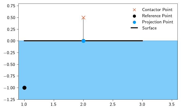
The target segment shall be the line segment connecting the points \((1, 0)\) and \((3, 0)\). The reference point inside the body to which the above line segment is a surface is \((0, -1)\)
We test the above implemented functions for 3 different contractor points:
\((2.0, 0.5)\)
\((3.5, 0.5)\)
\((2.0, -0.2)\)
Use the following code to test your implementation. Replace the contactor_point with the above points to test your implementation.
contactor_point = np.array([2, 0.5]) # Change this for different scenariossurface_coords = np.array([[1, 0], [3, 0.0]])reference_point = np.array([1, -1])normal = find_normal_to_surface(surface_coords, reference_point)projection_point = find_projection_point( contactor_point, surface_coords, normal)projected_distance, inside = find_distance_to_point( contactor_point, projection_point, surface_coords, normal)print("The normal to the surface is: ", normal)print("The projection point is: ", projection_point)print("The projected distance is: ", projected_distance)print("The inside flag is: ", inside)plt.style.use(STYLE_PATH)plt.figure(figsize=(5, 3), layout="constrained")ax = plt.axes()ax.scatter( contactor_point[0], contactor_point[1], marker="x", s=50, color=colors.red, zorder=10, label="Contactor Point",)ax.scatter( reference_point[0], reference_point[1], marker="o", s=50, color="k", zorder=10, label="Reference Point",)ax.fill_between(x=np.linspace(0.9, 3.6), y1=0, y2=-1.5, color=colors.blue, alpha=0.5)ax.scatter( projection_point[0], projection_point[1], marker="o", s=50, color=colors.blue, zorder=10, label="Projection Point",)ax.plot(surface_coords[:, 0], surface_coords[:, 1], lw=2, color="k", label="Surface")ax.plot( [contactor_point[0], projection_point[0]], [contactor_point[1], projection_point[1]], color="gray",)ax.set_xlim(0.9, 3.6)ax.set_ylim(-1.25, 0.8)ax.legend(frameon=False)plt.show()
The normal to the surface is:  [-0.  1.]
The projection point is:  [2. 0.]
The projected distance is:  0.5
The inside flag is:  1
Figure 13.1: Testing the implementation of contact detection for a single contactor point and a single target segment.
Step 4: Find the best valid point
This is the “search” step. For a single contactor node, we have a list of projected distances from all target segments. We need to filter this list and find the single “best” one (the closest and penetrating). Return the coords of the closest projection point and the normal of the corresponding segment.
Hint
The function implementation will look something like this
def find_valid_orthogonal_point( projected_distances: Array, inside: Array, projection_points: Array, surface_normals: Array,) -> Tuple[Array, Array]:""" Find the closest point and corresponding normal on a surface to a point. Args: projected_distances: The projected distances to the surface, shape (n,) inside: The inside flag, shape (n,) projection_points: The projection points, shape (n, 2) surface_normals: The normals at the surface points, shape (n, 2) Returns: closest_point: The closest point on the surface, shape (2,) closest_normal: The normal at the closest point, shape (2,) """return ...
@jax.jitdef find_valid_orthogonal_point( projected_distances: Array, inside: Array, projection_points: Array, surface_normals: Array,) -> Tuple[Array, Array]:""" Find the closest point and corresponding normal on a surface to a point. Args: projected_distances: The projected distances to the surface, shape (n,) inside: The inside flag, shape (n,) projection_points: The projection points, shape (n, 2) surface_normals: The normals at the surface points, shape (n, 2) Returns: closest_point: The closest point on the surface, shape (2,) closest_normal: The normal at the closest point, shape (2,) """ projected_distances = jnp.where( (inside ==1) & (projected_distances <0), projected_distances,-jnp.inf, ) index = jnp.argmax(projected_distances) closest_point = projection_points[index] closest_normal = surface_normals[index]return closest_point, closest_normal
Step 5: Putting it all together
Finally, orchestrate all the steps in the main find_gap function. This function will look like it’s written for a single contactor point, but @autovmap will ensure it works for an entire array of points. This function will make use all previously defined functions.
Hint
The function implementation will look something like this
@autovmap(contactor_point=1)def find_gap(contactor_point: Array, surface_points: Array, reference_points: Array) ->float:""" Find the gap between a point and a surface. The function returns the gap. Args: contactor_point: The point to find the gap to. surface_points: The coordinates of the nodes of the surface surface_normals: The normals at the nodes of the surface. Returns: gap: The closest gap between the point and the surface. """return ...
@autovmap(contactor_point=1)def find_gap(contactor_point: Array, surface_points: Array, reference_points: Array) ->float:""" Find the gap between a point and a surface. The function returns the gap. Args: contactor_point: The point to find the gap to. surface_points: The coordinates of the nodes of the surface. surface_normals: The normals at the nodes of the surface. Returns: gap: The closest gap between the point and the surface. """ surface_normals = find_normal_to_surface(surface_points, reference_points) projection_points = find_projection_point( contactor_point, surface_points, surface_normals ) projected_distances, inside = find_distance_to_point( contactor_point, projection_points, surface_points, surface_normals ) closest_point, closest_normal = find_valid_orthogonal_point( projected_distances, inside, projection_points=projection_points, surface_normals=surface_normals, ) gap = jnp.vdot(contactor_point - closest_point, closest_normal) gap = jnp.where(jnp.min(projected_distances) == jnp.inf, 0.0, gap)return gap
Testing the logic for multiple contactor nodes and multiple target segments
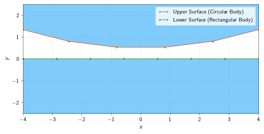
Now we will test the implemented algorithm for multiple contractor nodes and multiple target segments. Let us assume two surfaces of two different bodies.
The upper surface is part of circular body and the lower surface is part of a rectangular body.
We will test two cases:
Case 1: When the upper surface is the contact surface and the lower surface is the target surface.
Case 2: When the lower surface is the contact surface and the upper surface is the target surface.
Code: Generate the contact surfaces for the test cases
def generate_contact_surfaces( num_upper_segments=5, num_lower_segments=7, radius=10.0, width=8.0, initial_gap=0.5):""" Generates nodes and elements for an upper circular surface and a lower flat surface. Args: num_upper_segments: Number of line elements for the circular surface. num_lower_segments: Number of line elements for the flat surface. radius: Radius of the circular body. width: Width of the flat rectangular body. initial_gap: Initial vertical separation between the two bodies. Returns: A tuple containing: - upper_nodes (np.ndarray): Coordinates of nodes on the circular surface. - upper_elements (np.ndarray): Connectivity for the circular surface elements. - lower_nodes (np.ndarray): Coordinates of nodes on the flat surface. - lower_elements (np.ndarray): Connectivity for the flat surface elements. """# Position the circle's center so its bottom is at y=initial_gap center_y = radius + initial_gap# Calculate angles to span a portion of the circle max_angle = np.arcsin((width /2) / radius) angles = np.linspace(-max_angle, max_angle, num_upper_segments +1) upper_x = radius * np.sin(angles) upper_y = center_y - radius * np.cos(angles) upper_nodes = np.vstack([upper_x, upper_y]).T# Create line elements [(0, 1), (1, 2), ...] upper_elements = np.array([[i, i +1] for i inrange(num_upper_segments)])# Generate the lower flat surface lower_x = np.linspace(-width /2, width /2, num_lower_segments +1) lower_y = np.zeros_like(lower_x) # Position the surface at y=0 lower_nodes = np.vstack([lower_x, lower_y]).T# Create line elements lower_elements = np.array([[i, i +1] for i inrange(num_lower_segments)])return jnp.array(upper_nodes), jnp.array(upper_elements), jnp.array(lower_nodes), jnp.array(lower_elements)# Generate the geometryupper_nodes, upper_elements, lower_nodes, lower_elements = generate_contact_surfaces()plt.style.use(STYLE_PATH)plt.figure(figsize=(6, 3), layout='constrained')plt.plot(upper_nodes[:, 0], upper_nodes[:, 1], 'o-', color=colors.red, label='Upper Surface (Circular Body)')plt.plot(lower_nodes[:, 0], lower_nodes[:, 1], 'o-', color=colors.green, label='Lower Surface (Rectangular Body)')# Plot upper surface (circular)plt.fill_between(upper_nodes[:, 0], y1=upper_nodes[:, 1], y2=2.5, color=colors.blue, alpha=0.5)# Plot lower surface (flat)plt.fill_between(lower_nodes[:, 0], y1=lower_nodes[:, 1], y2=-2.5, color=colors.blue, alpha=0.5)plt.xlim(np.min(upper_nodes[:, 0]), np.max(upper_nodes[:, 0]))plt.ylim(-2.5, 2.5)plt.xlabel(r'$x$')plt.ylabel(r'$y$')plt.legend()plt.grid(True, linestyle='--', alpha=0.6)plt.show()
Figure 13.2: Contact surfaces for the test cases for the contact detection algorithm
Below we define two functions to plot the contact pairs. The first function check_contact_pairs is used to check the contact pairs between the contactor and the target surface. The second function plot_contact_pairs is used to plot the contact pairs. These functions are there just for visualization purposes and are not used in the algorithm.
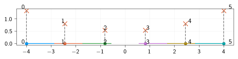
Case 1: Upper surface is the contact surface and the lower surface is the target surface
Let us check if the algorithm works for the case when the upper surface is the contact surface and the lower surface is the target surface. Both the surfaces are separated i.e there is no contact between the two surfaces. This means that the gap should be positive everywhere. Since the target surface is flat (\(n\) is [0, 1]) at y=0, the gap will be the \(y-\)coordinate of the contactor point.
Use the find_gap function that you implemented above to compute the gap between the contactor and the target surface.
Let us also visualize the contact pairs i.e the contactor points and the closest points on the target surface and the normals at the contact points. We use the plot_contact_pairs function to visualize the contact pairs.
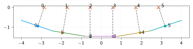
Figure 13.3: Contact pairs between the upper surface and the lower surface. Contactor points (upper surface) are marked with red crosses and the closest points on the target surface (lower surface) are marked with circles. The target surface is marked with the same color as the closest points.
Case 2: Lower surface is the contact surface and the upper surface is the target surface
Let us check if the algorithm works for the case when the lower surface is the contact surface and the upper surface is the target surface. Both the surfaces are separated i.e there is no contact between the two surfaces. This means that the gap should be positive everywhere. Since the target surface is flat (\(n\) is [0, 1]) at y=0, the gap will be the \(y-\)coordinate of the contactor point.
We also move the upper surface down by 2 units so that the two bodies are intersecting. Use the find_gap function that you implemented above to compute the gap between the contactor and the target surface.
Figure 13.4: Contact pairs between the lower surface and the upper surface. Contactor points (lower surface) are marked with red crosses and the closest points on the target surface (upper surface) are marked with circles. The target surface is marked with the same color as the closest points.
Defining the contact energy
Now we have a algorithm to compute the gap between a point and a surface. We can use this algorithm to compute the contact energy.
The contact energy is defined as:
\[
\Psi_\text{contact}(u)=\frac{1}{2}k_\text{pen}\int_{\Gamma_c}\langle -g(u)\rangle^2 \text{d}\Gamma
\] where \(\Gamma_c\) is the contact surface, \(k_\text{pen}\) is the penalty parameter, and \(g(u)\) is the gap function. The Macaluay’s bracket is defined as:
where \(N_c\) is the number of nodes on the contact surface, \(A_i\) is the area of the node \(i\), and \(g(u_i)\) is the gap function at node \(i\).
Defining the penalty parameter
The penalty parameter \(k_\text{pen}\) is a parameter that controls the stiffness of the contact. It is a scalar parameter that is used to penalize the violation of the contact constraint.
Below define the penalty parameter \(k_\text{pen}\).
k_pen =5.0
Computing the contact energy
Now we have all the ingredients to define the contact energy.
Below we define the function to compute the contact energy. This function is the same as the one defined in the previous exercise except for the fact, it also takes the reference points as an argument.
@jax.jitdef macalauy_bracket(x):return jnp.where(x >0, 0, x)@jax.jitdef compute_contact_energy( u: Array, coords: Array, contactor_nodes: Array, nodes_area: Array, target_surface_elements: Array, reference_points: Array,) -> Array:"""Compute the contact energy for a given displacement field. Args: u: Displacement field. coords: Coordinates of the nodes. contactor_nodes: Indices of the nodes on the contactor surface. nodes_area: Area of the nodes on the contactor surface. target_surface_elements: Coordinates of the points of target surface. reference_points: Coordinates of the reference points of the target surface. Returns: Contact energy. """ new_coords = coords + u points = new_coords[contactor_nodes] contactor_nodes_area = nodes_area[contactor_nodes] surface_points = new_coords[target_surface_elements]# Loop over nodes on the potential contact surfacedef _contact_energy_node(point, contact_area): gap = find_gap(point, surface_points, reference_points) gap = macalauy_bracket(gap)return0.5* k_pen * (gap**2) * contact_area contact_energy_node = jax.vmap(_contact_energy_node, in_axes=(0, 0))return jnp.sum(contact_energy_node(points, contactor_nodes_area))
The One-Pass Algorithm (The Biased Approach)
In the above function to compute the contact energy, we have to make a choice: which body is the “contactor” and which is the “target”? It turns out this seemingly arbitrary choice can introduce a significant bias into the simulation, leading to unphysical results.
In order to understand how the bias is introduced, let us consider a simple example, contact between a triangular surface and a flat surface. For simplicity, we consider two line elements on the triangular surface and one line element on the flat surface.
Lets us first consider the case when the triangular surface is the contactor and the flat surface is the target. Below we define some trial nodes and elements to represent the triangular and flat surfaces. We also define a trial displacement field to represent the displacement of the nodes. The displacement is such that the triangular surface is pushed into the flat surface.
Below we define a function to compute the contact energy \(\Psi_\text{contact}\) when the triangular surface is the contactor and the flat surface is the target. We make use of the compute_contact_energy function defined above. We compute the contact force that will be exerted on the nodes of both the surfaces due to the interpenetration.
We plot these contact forces on the nodes of the both surfaces. As expected the direction of the contact force is determined by the direction of the normal to the target surface.
Code: Compute the contact energy and the contact force when the triangular surface is the contactor and the flat surface is the target
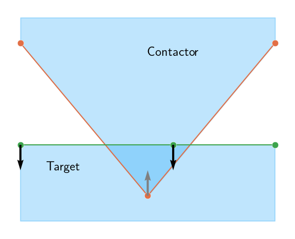
Figure 13.5: Contact forces on the nodes of the triangular and flat surfaces when the triangular surface is the contactor and the flat surface is the target.
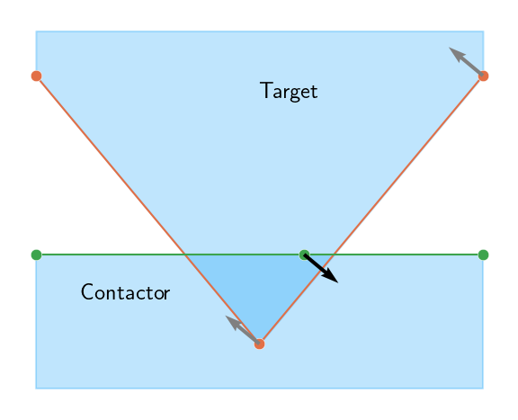
Next, we consider the case when the flat surface is the contactor and the triangular surface is the target. We repeat the same steps as above to compute the contact energy and the contact force. Upon plotting the contact forces, we observe that the contact forces are in different direction compared to the case when the triangular surface is the contactor. This is because the direction of the contact force is determined by the direction of the normal to the target surface. Earlier, the normal was pointing outwards the flat surface and now it is pointing outwards the triangular surface.
This is exactly the cause of the bias in the contact force.
Code: Compute the contact energy and the contact force when the flat surface is the contactor and the triangular surface is the target
Figure 13.6: Contact forces on the nodes of the triangular and flat surfaces when the flat surface is the contactor and the triangular surface is the target.
The One-Pass Algorithm (The Biased Approach)
The above approach for selecting one contactor surface and one target surface is called the one-pass algorithm. As shown above, this approach is biased and can lead to unphysical results. Therefore, when we are dealing with contact of deformable bodies, we use a two-pass or symmetrized approach.
The Two-Pass Algorithm (The Symmetrized Approach)
To eliminate this bias and create a robust algorithm, we use a two-pass or symmetrized approach. The logic is simple but powerful: we perform the contact check twice, swapping the roles of the bodies each time.
Pass 1: Treat Body A as the contactor and Body B as the target. Calculate the contact penalty energy based on any penetrations found (\(\Psi_{A \to B}\)).
Pass 2: Swap the roles. Now treat Body B as the contactor and Body A as the target. Calculate a separate contact penalty energy (\(\Psi_{B \to A}\)).
Combine: The total contact energy is the average of the two passes: \[\Psi_{\text{contact}} = \frac{1}{2} (\Psi_{A \to B} + \Psi_{B \to A})\]
By performing two passes, we ensure that no matter which body’s nodes are penetrating the other’s segments, a resisting penalty force will always be generated. This symmetrization eliminates the bias and leads to a much more accurate and physically realistic simulation, especially when the two bodies have similar mesh densities or complex geometries
Below, we define the functions to compute the contact energy and the contact force using the two-pass algorithm.
Code: Compute the contact energy using the two-pass algorithm
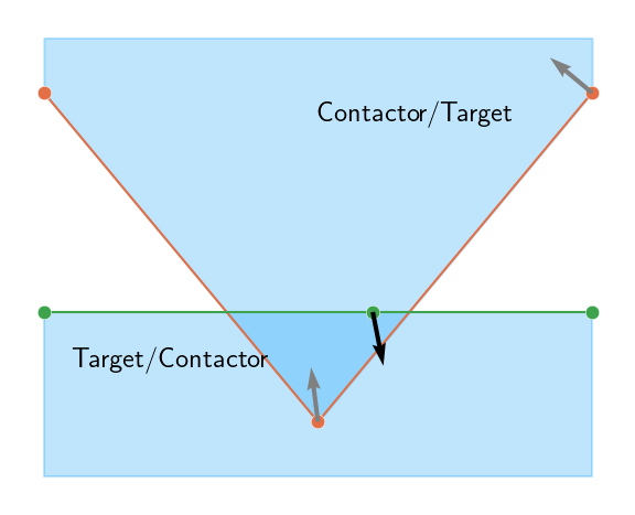
Figure 13.7: Contact forces on the nodes of the triangular and flat surfaces using the two-pass algorithm
Important
The grading of the assignment will be based on the correctness of the algorithm. The part below will not be considered for grading. However, we encourage you to also go through the part below as it uses the algorithm implemented above and solve the problem of contact between two deformable bodies.
Please go through the part below to understand the problem statement and the solution.
Model setup
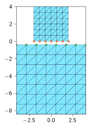
Next, we use the contact detection algorithm and the concept of two-pass algorithm to resolve the contact between two deformable bodies. Below, we generate a triangular mesh of a half-circle. We also define a function to get the elements and nodes on the potential contact surface.
Code: Functions to generate the mesh
def generate_block_mesh( nx: int, ny: int, lxs: Tuple[float, float], lys: Tuple[float, float], curve_func: Optional[Callable[[Array, float], bool]] =None, tol: float=1e-6,) -> Tuple[Array, Array, Optional[Array]]:""" Generates a 2D triangular mesh for a rectangle and optionally extracts 1D line elements along a specified curve. Args: nx: Number of elements along the x-direction. ny: Number of elements along the y-direction. lxs: Tuple of the x-coordinates of the left and right edges of the rectangle. lys: Tuple of the y-coordinates of the bottom and top edges of the rectangle. curve_func: An optional callable that takes a coordinate array [x, y] and a tolerance, returning True if the point is on the curve. tol: Tolerance for floating-point comparisons. Returns: A tuple containing: - coords (jnp.ndarray): Nodal coordinates, shape (num_nodes, 2). - elements_2d (jnp.ndarray): 2D triangular element connectivity. - elements_1d (jnp.ndarray | None): 1D line element connectivity, or None. """ x = jnp.linspace(lxs[0], lxs[1], nx +1) y = jnp.linspace(lys[0], lys[1], ny +1) xv, yv = jnp.meshgrid(x, y, indexing="ij") coords = jnp.stack([xv.ravel(), yv.ravel()], axis=-1)def node_id(i, j):return i * (ny +1) + j elements_2d = []for i inrange(nx):for j inrange(ny): n0 = node_id(i, j) n1 = node_id(i +1, j) n2 = node_id(i, j +1) n3 = node_id(i +1, j +1) elements_2d.append([n0, n1, n3]) elements_2d.append([n0, n3, n2]) elements_2d = jnp.array(elements_2d)# --- 2. Extract 1D elements if a curve function is provided ---if curve_func isNone:return coords, elements_2d, None# Efficiently find all nodes on the curve using jax.vmap on_curve_mask = jax.vmap(lambda c: curve_func(c, tol))(coords) elements_1d = []# Iterate through all 2D elements to find edges on the curvefor tri in elements_2d:# Define the three edges of the triangle edges = [(tri[0], tri[1]), (tri[1], tri[2]), (tri[2], tri[0])]for n_a, n_b in edges:# If both nodes of an edge are on the curve, add it to the setif on_curve_mask[n_a] and on_curve_mask[n_b]:# Sort to store canonical representation, e.g., (1, 2) not (2, 1) elements_1d.append(tuple(sorted((n_a, n_b))))ifnot elements_1d:return coords, elements_2d, jnp.array([], dtype=int)return coords, elements_2d, jnp.unique(jnp.array(elements_1d), axis=0)def generate_two_blocks_mesh( upper_ns: Tuple[int, int], lower_ns: Tuple[int, int], upper_lengths: Tuple[float, float], lower_lengths: Tuple[float, float], gap: float, upper_curve_func: Callable[[Array, float], bool], lower_curve_func: Callable[[Array, float], bool], tol: float=1e-6,) -> Tuple[Array, Array, Optional[Array]]:""" Generates a 2D triangular mesh for two blocks and optionally extracts 1D line elements along a specified curve. Args: nx: Number of elements along the x-direction. ny: Number of elements along the y-direction. lxs: Tuple of the x-coordinates of the left and right edges of the rectangle. lys: Tuple of the y-coordinates of the bottom and top edges of the rectangle. curve_func: An optional callable that takes a coordinate array [x, y] and a tolerance, returning True if the point is on the curve. tol: Tolerance for floating-point comparisons. Returns: A tuple containing: - coords (jnp.ndarray): Nodal coordinates, shape (num_nodes, 2). - elements_2d (jnp.ndarray): 2D triangular element connectivity. - elements_1d (jnp.ndarray | None): 1D line element connectivity, or None. """ upper_nx, upper_ny = upper_ns lower_nx, lower_ny = lower_ns upper_lx, upper_ly = upper_lengths lower_lx, lower_ly = lower_lengths upper_coords, upper_elements_2d, upper_elements_1d = generate_block_mesh( nx=upper_nx, ny=upper_ny, lxs=(-upper_lx/2, upper_lx/2), lys=(0, upper_ly), curve_func=upper_curve_func, tol=tol ) lower_coords, lower_elements_2d, lower_elements_1d = generate_block_mesh( nx=lower_nx, ny=lower_ny, lxs=(-lower_lx/2, lower_lx/2), lys=(-(lower_ly+gap), -gap), curve_func=lower_curve_func, tol=tol ) coords = jnp.vstack((upper_coords, lower_coords)) elements = jnp.vstack( (upper_elements_2d, lower_elements_2d + upper_coords.shape[0]) ) mesh = Mesh(coords, elements) lower_elements_1d = lower_elements_1d + upper_coords.shape[0]return ( mesh, upper_elements_2d, lower_elements_2d + upper_coords.shape[0], upper_elements_1d, lower_elements_1d, )
upper_ns = (6, 6) # Number of elements in Xlower_ns = (7, 7) # Number of elements in Yupper_lengths = (4, 4)lower_lengths = (8, 8)gap =0.4# initial gap between bodies# function to identify the potential contact elements on the upper bodydef upper_block_line(coord: Array, tol: float) ->bool:return jnp.logical_and(jnp.isclose(coord[1], 0.0, atol=tol), coord[0] >=-upper_lengths[0])# function to identify the potential contact elements on the lower bodydef lower_block_line(coord: Array, tol: float) ->bool:return jnp.logical_and(jnp.isclose(coord[1], -gap, atol=tol), coord[0] >=-lower_lengths[0])( mesh, upper_elements, lower_elements, upper_contact_elements, lower_contact_elements,) = generate_two_blocks_mesh( upper_ns=upper_ns, lower_ns=lower_ns, upper_lengths=upper_lengths, lower_lengths=lower_lengths, gap=gap, upper_curve_func=upper_block_line, lower_curve_func=lower_block_line,)# get the nodes from the contact elementsupper_contact_nodes = jnp.unique(upper_contact_elements.flatten())lower_contact_nodes = jnp.unique(lower_contact_elements.flatten())n_nodes = mesh.coords.shape[0]n_dofs_per_node =2n_dofs = n_dofs_per_node * n_nodes
tri = element.Tri3()op = Operator(mesh, tri)mat = Material(mu=mu, lmbda=lmbda)@autovmap(grad_u=2)def compute_strain(grad_u: Array) -> Array:"""Compute the strain tensor from the gradient of the displacement."""return0.5* (grad_u + grad_u.T)@autovmap(eps=2)def compute_stress(eps: Array, mu: float, lmbda: float) -> Array:"""Compute the stress tensor from the strain tensor.""" I = jnp.eye(2)return2* mu * eps + lmbda * jnp.trace(eps) * I@autovmap(grad_u=2)def strain_energy(grad_u: Array, mu: float, lmbda: float) -> Array:"""Compute the strain energy density.""" eps = compute_strain(grad_u) sig = compute_stress(eps, mu, lmbda)return0.5* jnp.einsum("ij,ij->", sig, eps)@jax.jitdef total_strain_energy(u_flat: Array) ->float:"""Compute the total energy of the system.""" u = u_flat.reshape(-1, n_dofs_per_node) grad_u = op.grad(u)return op.integrate(strain_energy(grad_u, mat.mu, mat.lmbda))
Defining contact energy
We will now define the contact energy using the two-pass algorithm. Use the function compute_contact_energy to compute the contact energy for \(\Psi_{A \to B}\) and \(\Psi_{B \to A}\) and average the two to get the total contact energy.
Below we define the function to compute the area associated with each contact node for the upper contact surface as well as the lower contact surface. Use these two vectors to compute the total contact energy.
Computing the area associated with each contact node
For correct resolution of the contact problem, we need the area associated with each contact node. In order to compute the area of each contact node, we define a line mesh that contains the contact nodes and the edges of the contact elements. We then define a function which integrates a constant field of value 1 over the line mesh.
where \(q(x)\) is a constant field of value 1. We can then compute the area of each node by differentiating the total area with respect to the field \(q(x)\).
def total_energy( u_flat: Array, coords: Array, ...) ->float:"""Compute the total energy for a given displacement field. Args: u_flat: Flattened displacement field, shape (n_dofs,). coords: Initial coordinates of the nodes, shape (n_nodes, 2). ... Other arguments need to be passed to the compute_contact_energy function for each body. Returns: Total energy, a scalar """# TODO: reshape the displacement field ...# TODO compute the total contact energy using two-pass algorithm contact_energy = ...# TODO compute the elastic energy strain_energy = ...# TODO Sum the contact and strain energies to get the total energy of the system.return ...
@jax.jitdef _total_energy( u_flat: Array, coords: Array,) -> Array:"""Compute the total energy for a given displacement field. Args: u_flat: Flattened displacement field. coords: Coordinates of the nodes. contact_nodes: Indices of the nodes on the contact surface. Returns: Total energy. """ u = u_flat.reshape(-1, n_dofs_per_node) upper_contact_energy = contact_energy_upper(u) lower_contact_energy = contact_energy_lower(u) contact_energy =0.5* (upper_contact_energy + lower_contact_energy) strain_energy = total_strain_energy(u)return strain_energy + contact_energytotal_energy = partial( _total_energy, coords=mesh.coords,)
Applying Dirichlet boundary conditions
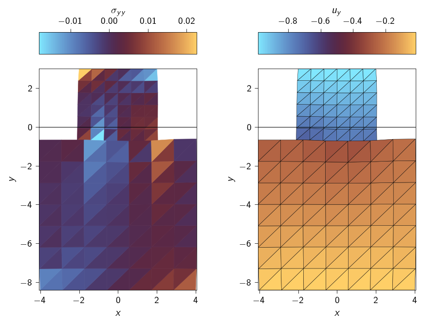
We push the upper deformable body into the lower deformable body by applying a displacement in the \(y\) direction on the top edge of the upper body. To avoid rigid body motion, we fix the displacement in the \(x\) direction on the top edge of the upper body. The lower body is fixed on the bottom edge in both the \(x\) and \(y\) directions.
The boundary conditions thus applied are:
\[
\begin{aligned}
u_x &= 0 \quad \text{on the top edge of the upper body} \\
u_y &= -1.0 \quad \text{on the top edge of the upper body} \\
u_x &= 0 \quad \text{on the bottom edge of the lower body} \\
u_y &= 0 \quad \text{on the bottom edge of the lower body} \\
\end{aligned}
\]
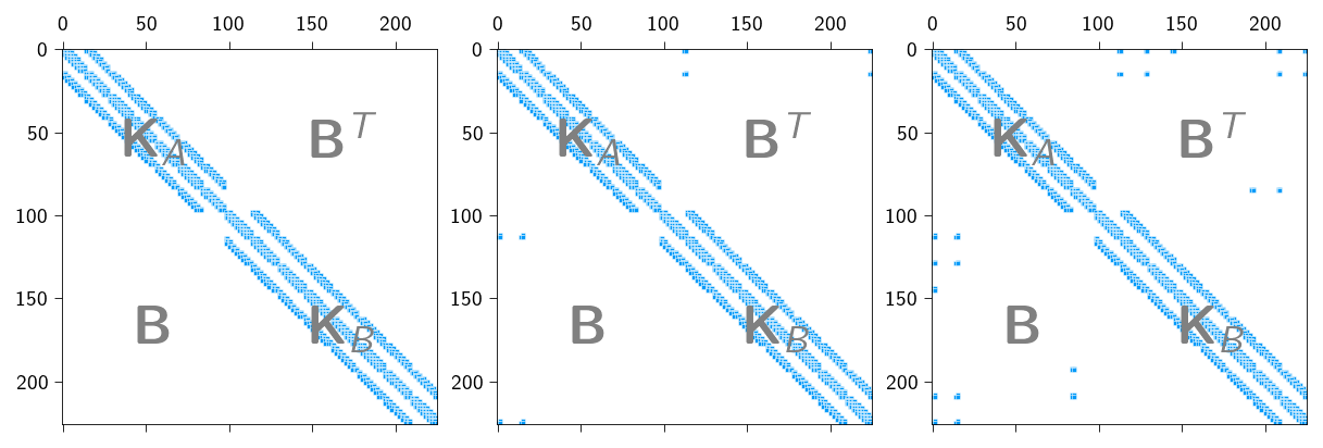
Since the contact pair (a contractor node and its closet target surface element) can change on every iteration, we need to use a more sophisticated solver than the one used in the last exercise. Below, we present the sparsity pattern for the above problem at 3 different time instants. The off-diagonal terms are due to the contact constraints between the two bodies. We can see that the sparsity pattern is changing as the contact pairs are changing. Initially, there are no contact constraints and the sparsity pattern is the same as the one for the linear elastic problem. As the contact starts, the sparsity pattern changes and the contact constraints are included in the stiffness matrix. Depending on which node is in contact, the sparsity pattern changes.
Figure 13.9: The sparsity pattern due to contact constraints at different time during loading. Left: initial configuration. Middle: at 80% of the applied displacement. Right: at 100% of the applied displacement.
Instead of buidling sparsity pattern again and again, we can make use of the matrix-free solvers (see Matrix-free solvers) to solve the linear system. In matrix-free solvers, we do not need to build the stiffness matrix explicitly. We can directly apply the stiffness operator to the displacement vector to get the residual. Then one can use the conjugate gradient method to solve the linear system.
Note
You might be wondering why we were building the stiffness matrix in the the last exercises. The reason is that all the last exercises we did were forming a KKT system of equations. If you recall, the KKT system of equations is of the form:
\[
\begin{bmatrix}
\mathbf{K} & \mathbf{B}^T \\
\mathbf{B} & \mathbf{0}
\end{bmatrix}
\begin{bmatrix}
\boldsymbol{u} \\
\boldsymbol{\lambda}
\end{bmatrix} = \begin{bmatrix} \boldsymbol{f} \\ \boldsymbol{0} \end{bmatrix}
\] And such systems are not positive definite (because of the \(\mathbf{0}\) block) and hence we needed a direct solver to solve the linear system. Conjugate gradient method, on the other hand, is applicable to positive definite systems and therefore, we never used matrix-free solvers.
While solving any constrained problem using Penalty methods, we never form a KKT system. For example, in the case of contact, we form a system of the form:
Notice, there is no \(\mathbf{0}\) block in the above form.
Below, we define the functions to compute the gradient and the Jacobian-vector product. Within the Jacoboian-Vector product we apply Lifting approach by first “zeroing” out the displacements and then “zeroing” out the residual at the fixed DOFs.
# creating functions to compute the gradient andgradient = jax.jacrev(total_energy)# create a function to compute the JVP product@jax.jitdef compute_tangent(du, u_prev): du_projected = du.at[fixed_dofs].set(0.0) tangent = jax.jvp(gradient, (u_prev,), (du_projected,))[1] tangent = tangent.at[fixed_dofs].set(0)return tangent
Below we define the Conjugate-gradient method and the Newton-Rahpson method to solve the nonlinear problem of contact.
Code: Functions to implement the conjugate gradient method and Newton-Rahpson method
def conjugate_gradient(A, b, atol=1e-8, max_iter=100): iiter =0def body_fun(state): b, p, r, rsold, x, iiter = state Ap = A(p) alpha = rsold / jnp.vdot(p, Ap) x = x + jnp.dot(alpha, p) r = r - jnp.dot(alpha, Ap) rsnew = jnp.vdot(r, r) p = r + (rsnew / rsold) * p rsold = rsnew iiter = iiter +1return (b, p, r, rsold, x, iiter)def cond_fun(state): b, p, r, rsold, x, iiter = statereturn jnp.logical_and(jnp.sqrt(rsold) > atol, iiter < max_iter) x = jnp.full_like(b, fill_value=0.0) r = b - A(x) p = r rsold = jnp.vdot(r, p) b, p, r, rsold, x, iiter = jax.lax.while_loop( cond_fun, body_fun, (b, p, r, rsold, x, iiter) )return x, iiterdef newton_krylov_solver( u, fext, gradient, compute_tangent, fixed_dofs,): fint = gradient(u) du = jnp.zeros_like(u) iiter =0 norm_res =1.0 tol =1e-8 max_iter =10while norm_res > tol and iiter < max_iter: residual = fext - fint residual = residual.at[fixed_dofs].set(0) A = jax.jit(partial(compute_tangent, u_prev=u)) du, cg_iiter = conjugate_gradient(A=A, b=residual, atol=1e-8, max_iter=100) u = u.at[:].add(du) fint = gradient(u) residual = fext - fint residual = residual.at[fixed_dofs].set(0) norm_res = jnp.linalg.norm(residual)print(f" Residual: {norm_res:.2e}") iiter +=1return u, norm_res
Implementing the Incremental Loading Loop
Now that we have the mesh, the energy functions, and the newton_krylov_solver, it’s time to set up the main simulation loop. We will apply the displacement in small increments and solve for equilibrium at each step. This is important because using penalty method, the problem becomes non-linear and the solution is sensitive to the initial guess.
Follow these steps to build the main part of your script.
Hint
Initialization
Before the loop, you need to initialize all the variables for the simulation.
Create the initial solution vector u_prev, which contains both displacements. Initialize it as a vector of zeros with the correct total size (n_dofs).
Initialize the external force vector fext as a vector of zeros.
Set the number of load increments, n_steps (e.g., 20). We would apply the total applied_displacement in n_steps.`
Calculate the displacement to apply at each step.
The Main Loading Loop
Create a for loop that iterates through each load step.
for step inrange(n_steps):print(f"Step {step+1}/{n_steps}")# ... Your code for each step will go inside this loop ...
Inside the Loop: Apply Displacement and Prepare Solver
At the beginning of each loop iteration, you need to update the boundary conditions and prepare the functions for the solver.
Update the u_prev vector with the prescribed displacement for the current step.
Inside the Loop: Solve for Equilibrium
Call the newton_krylov_solver function with the initial guess and other arguments. Depending on what inputs your gradient and compute_tangent functions require, you may need to pass additional arguments to the newton_krylov_solver function. You will also have to pass the fixed_dofs to the newton_krylov_solver function to apply the lifting method.
Store the new solution in u_new.
Update the state for the next iteration by setting u_prev = u_new. This is basically providing the solution from the previous step as the initial guess for the next step., which helps the solver converge faster.
After the Loop: Final Solution
Once the loop is complete, extract the final displacement field from the final u_prev vector for visualization.