In this exercise, we will study and analyze the crack propagation under dynamic conditions. The case when the crack propagation is no longer quasi-static, but dynamic. Unlike, quasi-static fracture, a dynamic crack propagation means that we can no longer neglect the inertial terms in the equations of motion.
We simulate the dynamic propagation of a crack in a pre-strained plate. To ensure a controlled initiation and isolate the effects of inertia, we split the simulation into two distinct phases:
Phase 1: Quasi-static Pre-loading
First, we stretch the plate slowly to a critical displacement. We solve for the equilibrium state where internal forces balance external loads, ignoring time and inertia.
Interface Model: The potential crack path is tied together using a stiff penalty (binding) potential. This prevents separation but allows us to store elastic energy in the bulk material without triggering crack propagation.
Energy Balance: The solver minimizes the total potential energy: \[\Psi_{\text{static}} = \Psi_{\text{elastic}}(\boldsymbol{u}) + \Psi_{\text{penalty}}(\boldsymbol{u})\]
This is nothing but constraining the two surfaces of the crack to not separate and we have seen such problem in various previous exercises.
Phase 2: Dynamic Propagation
Once the plate is pre-loaded, we fix the displacement boundaries (clamped condition) and switch the solver to an explicit dynamic time-integration. We simultaneously switch the interface model to an reversible cohesive law. The crack is now free to propagate, driven solely by the release of stored strain energy.
Interface Model: An exponential cohesive zone model that dissipates energy as the surfaces separate.
Energy Balance: The total energy of the system must be conserved. The stored elastic potential is converted into kinetic energy (stress waves) and dissipated fracture energy: \[E_{\text{total}} = \underbrace{T_{\text{kinetic}}(\dot{\boldsymbol{u}})}_{\text{Inertia}} + \underbrace{\Psi_{\text{elastic}}(\boldsymbol{u})}_{\text{Stored}} + \underbrace{\Psi_{\text{fracture}}(\boldsymbol{u})}_{\text{Dissipated}} = \text{Constant}\]
Objective: We will track the conversion of \(\Psi_{\text{elastic}}\) into \(\Psi_{\text{fracture}}\) and observe the role of \(E_{\text{kinetic}}\) in limiting the crack tip velocity.
Let us start by importing the necessary libraries and modules. We will use the same libraries as in the previous exercise.
Code: Import essential libraries
import jaxjax.config.update("jax_enable_x64", True) # use double-precisionjax.config.update("jax_persistent_cache_min_compile_time_secs", 0)jax.config.update("jax_platforms", "cpu")import jax.numpy as jnpfrom jax import Arrayfrom tatva import Mesh, Operator, elementfrom tatva.plotting import STYLE_PATH, colors, plot_element_values, plot_nodal_valuesfrom jax_autovmap import autovmapimport equinox as eqximport numpy as npfrom typing import Callable, Optional, Tupleimport matplotlib.pyplot as plt
Model Setup
We use the same configuration and material properties as in In-class activity: Quasistatic fracture. We will load the plate under Mode-I loading quasi-statically without letting the crack to propagate. This is analogous to loading the plate until it reaches the critical load for crack propagation. One can think of this situation as that before the crack starts propagating, how it reaches the critical load is not relevant. Since we want to study what happens to a crack propagating under dynamic loading, we can neglect the effect of the loading prior to the crack propagation.
mu: 39259.259259259255 N/m^2
lmbda: 91604.93827160491 N/m^2
L_G: 0.0051332024864342955 m
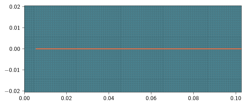
Using the above dimensions, we define a domain of length \(20\times L_G\) and height \(8\times L_G\). The plate has a pre-crack of length slightly larger than the Griffith fracture length \(L_G\).
For this exercise, we will use a pre-crack length of \(1.0\times L_G\). We use triangular elements to discretize the domain.
Code: Functions to generate the mesh
def generate_mesh_with_line_elements( nx: int, ny: int, lxs: Tuple[float, float], lys: Tuple[float, float], curve_func: Optional[Callable[[Array, float], bool]] =None, tol: float=1e-6,) -> Tuple[Array, Array, Optional[Array]]:""" Generates a 2D triangular mesh for a rectangle and optionally extracts 1D line elements along a specified curve. Args: nx: Number of elements along the x-direction. ny: Number of elements along the y-direction. lxs: Tuple of the x-coordinates of the left and right edges of the rectangle. lys: Tuple of the y-coordinates of the bottom and top edges of the rectangle. curve_func: An optional callable that takes a coordinate array [x, y] and a tolerance, returning True if the point is on the curve. tol: Tolerance for floating-point comparisons. Returns: A tuple containing: - coords (jnp.ndarray): Nodal coordinates, shape (num_nodes, 2). - elements_2d (jnp.ndarray): 2D triangular element connectivity. - elements_1d (jnp.ndarray | None): 1D line element connectivity, or None. """ x = jnp.linspace(lxs[0], lxs[1], nx +1) y = jnp.linspace(lys[0], lys[1], ny +1) xv, yv = jnp.meshgrid(x, y, indexing="ij") coords = jnp.stack([xv.ravel(), yv.ravel()], axis=-1)def node_id(i, j):return i * (ny +1) + j elements_2d = []for i inrange(nx):for j inrange(ny): n0 = node_id(i, j) n1 = node_id(i +1, j) n2 = node_id(i, j +1) n3 = node_id(i +1, j +1)#elements_2d.append([n0, n1, n3])#elements_2d.append([n0, n3, n2]) elements_2d.append([n0, n1, n2]) elements_2d.append([n1, n3, n2]) elements_2d = jnp.array(elements_2d)# --- 2. Extract 1D elements if a curve function is provided ---if curve_func isNone:return coords, elements_2d, None# Efficiently find all nodes on the curve using jax.vmap on_curve_mask = jax.vmap(lambda c: curve_func(c, tol))(coords) elements_1d = []# Iterate through all 2D elements to find edges on the curvefor tri in elements_2d:# Define the three edges of the triangle edges = [(tri[0], tri[1]), (tri[1], tri[2]), (tri[2], tri[0])]for n_a, n_b in edges:# If both nodes of an edge are on the curve, add it to the setif on_curve_mask[n_a] and on_curve_mask[n_b]:# Sort to store canonical representation, e.g., (1, 2) not (2, 1) elements_1d.append(tuple(sorted((n_a, n_b))))ifnot elements_1d:return coords, elements_2d, jnp.array([], dtype=int)return coords, elements_2d, jnp.unique(jnp.array(elements_1d), axis=0)
Nx =200# Number of elements in XNy =40# Number of elements in YLx =20* L_G # Length in XLy =8* L_G # Length in Ycrack_length =1.0* L_G# function identifies nodes on the cohesive line at y = 0. and x > 2.0def cohesive_line(coord: Array, tol: float) ->bool:return jnp.logical_and( jnp.isclose(coord[1], 0.0, atol=tol), coord[0] > crack_length )upper_coords, upper_elements_2d, top_interface_elements = generate_mesh_with_line_elements( nx=Nx, ny=Ny, lxs=(0, Lx), lys=(0, Ly/2), curve_func=cohesive_line)lower_coords, lower_elements_2d, bottom_interface_elements = generate_mesh_with_line_elements( nx=Nx, ny=Ny, lxs=(0, Lx), lys=(-Ly/2, 0), curve_func=cohesive_line)coords = jnp.vstack((upper_coords, lower_coords))elements = jnp.vstack((upper_elements_2d, lower_elements_2d + upper_coords.shape[0]))mesh = Mesh(coords, elements)n_nodes = mesh.coords.shape[0]n_dofs_per_node =2n_dofs = n_dofs_per_node * n_nodesbottom_interface_elements = bottom_interface_elements + upper_coords.shape[0]
We start with the quasi-static pre-loading phase. Here, we will apply a displacement boundary condition to the top and the bottom edge of the plate to stretch it in the vertical direction. We will use a stiff penalty potential along the cohesive line to prevent crack propagation during this phase.
Defining the penalty energy density to tie the crack surfaces
The constraint to prevent the two surfaces of the crack from separating is given as
Now to constraint the two surfaces of the crack from separating, we define a penalty energy density based on the displacement jump across the interface.
The penalty energy is defined as: \[
\Psi_{\text{penalty}} = \frac{1}{2} \int \underbrace{\kappa_{\text{penalty}} (g(\boldsymbol{u}))^2}_{\psi_{\text{penalty}}} d\Gamma
\]
where
\(\Gamma_{coh}\) is the cohesive interface.
\(\kappa_\text{binding}\) is the penalty stiffness parameter that controls the strength of the constraint.
To compute the total penalty energy, we will integrate the penalty energy density over the cohesive interface. So we need two things:
A line integral over the cohesive interface.
The penalty energy density function \(\psi_{\text{penalty}}\).
Defining the operator for line integration
We will begin by defining the operator for line integration similar to Operator that we have used for the triangular elements. To do so, we will have to first define the line elements along the potential fracture surface. We will use the Line2 element to define the line elements. This element has 2 nodes. Below, we use the function extract_interface_mesh to generate the mesh that consists of the line elements along the potential fracture surface. Since the two interfaces are discretized using the same number of elements, and occupy the same spatial domain, we can use any one of the two to perform the integration.
Code: Extract the interface mesh
def extract_interface_mesh(mesh, line_elements):"""Generate a mesh for the interface between two materials."""# --- Interface mesh --- line_element_nodes = jnp.unique(line_elements.flatten()) interface_coords = mesh.coords[line_element_nodes] interface_elements = jnp.array( [[index, index +1] for index inrange(len(line_elements))] ) interface_mesh = Mesh(interface_coords, interface_elements)return interface_mesh
Define the function below to compute the penalty energy density.
@jax.jitdef safe_sqrt(x):return jnp.sqrt(jnp.where(x >0.0, x, 0.0))@autovmap(jump=1)def compute_opening(jump: Array) ->float:""" Compute the opening of the cohesive element. Args: jump: The jump in the displacement field. Returns: The opening of the cohesive element. """ opening = safe_sqrt(jump[0] **2+ jump[1] **2)return opening@autovmap(jump=1)def binding_energy(jump: Array, binding_penalty=1e8) ->float:""" Compute the binding energy of the cohesive element. Args: jump: The jump in the displacement field. Returns: The binding energy of the cohesive element. """ delta = compute_opening(jump)return0.5* binding_penalty * delta**2
Now use the above defined function and the line_op operator to compute the penelty energy to tie the two surfaces of the crack. The penalty energy is then given by:
We will need the nodes associated with the interface elements to later compute the effefctive opening between the lower and upper bodies across the crack.
Below get the nodes from the bottom and top interfaces.
Once you have the nodes from the bottom and top interfaces, you can define the function to compute the penalty energy to constrain the two surfaces of the crack.
Finally, we can put everything together to compute the total energy. The total potential energy \(\Psi\) is the sum of the elastic strain energy \(\Psi_{elastic}\) and the penalty energy \(\Psi_\text{penalty}\).
Now lets us use the function defined above to compute the total energy of the system. This is just to check that there is no implementation error in the way we coded the functions above.
Applying Boundary Conditions
We now locate the dofs in the two domains to apply boundary conditions. We load the domain under Model I loading where both the top and bottom surfaces are loaded along the \(y\)-direction only. Furthermore, we assume symmetry about the \(x\)-axis at the left edge of the domain. Under symmetry, the domain represents a thorough crack in the middle of the domain. So the boundary conditions are:
\(u_x = 0\) on the left edge
\(u_y = -H\varepsilon_0/2\) on the bottom edge
\(u_y = H\varepsilon_0/2\) on the top edge
\(u_x = 0\) on the top and bottom edges
where \(H\) is the height of the domain and \(\varepsilon_0\) is the applied prestrain.
Now, we define a few functions to implement the matrix-free solvers. We will use the conjugate gradient method to solve the linear system of equations. The Dirichlet boundary conditions are applied using projection method. As we use the matrix-free solver, we need to define the gradient of the total potential energy, which is also the residual function.
Below define the function to compute the \(\boldsymbol{f}_{int}\) using jax.jacrev and then use this function to compute the Jacobian-vector product using jax.jvp. Remember to apply the Projection approach to enforce the Dirichlet boundary conditions.
gradient_static = jax.jacrev(total_static_energy)# create a function to compute the JVP product@jax.jitdef compute_tangent(du, u_prev): du_projected = du.at[fixed_dofs].set(0) tangent = jax.jvp(gradient_static, (u_prev,), (du_projected,))[1] tangent = tangent.at[fixed_dofs].set(0)return tangent
Code: Functions to implement the conjugate gradient method and Netwon-Raphson method
@eqx.filter_jitdef conjugate_gradient(A, b, atol=1e-8, max_iter=100): iiter =0def body_fun(state): b, p, r, rsold, x, iiter = state Ap = A(p) alpha = rsold / jnp.vdot(p, Ap) x = x + jnp.dot(alpha, p) r = r - jnp.dot(alpha, Ap) rsnew = jnp.vdot(r, r) p = r + (rsnew / rsold) * p rsold = rsnew iiter = iiter +1return (b, p, r, rsold, x, iiter)def cond_fun(state): b, p, r, rsold, x, iiter = statereturn jnp.logical_and(jnp.sqrt(rsold) > atol, iiter < max_iter) x = jnp.full_like(b, fill_value=0.0) r = b - A(x) p = r rsold = jnp.vdot(r, p) b, p, r, rsold, x, iiter = jax.lax.while_loop( cond_fun, body_fun, (b, p, r, rsold, x, iiter) )return x, iiterdef newton_krylov_solver( u, fext, gradient, fixed_dofs,): fint = gradient(u) du = jnp.zeros_like(u) iiter =0 norm_res =1.0 tol =1e-8 max_iter =50while norm_res > tol and iiter < max_iter: residual = fext - fint residual = residual.at[fixed_dofs].set(0) A = eqx.Partial(compute_tangent, u_prev=u) du, cg_iiter = conjugate_gradient(A=A, b=residual, atol=1e-8, max_iter=100) u = u.at[:].add(du) fint = gradient(u) residual = fext - fint residual = residual.at[fixed_dofs].set(0) norm_res = jnp.linalg.norm(residual)print(f" Residual: {norm_res:.2e}") iiter +=1return u, norm_res
Implementing the Incremental Loading Loop
We now run the simulation for \(\varepsilon_{applied} = 0.7 \times \varepsilon^0\).
The entire loading is divided into 10 increments At each increment, we solve the Newton-Krylov system using the conjugate gradient method. After each increment, we store the displacement and the force on the top surface.
Force-displacement response and deformed configuration
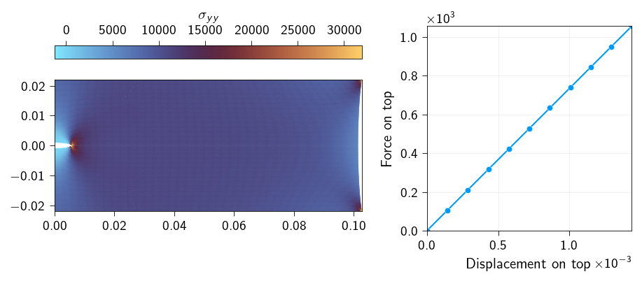
Let us now plot the force-displacement curve. This is the curve that we get by plotting the force on the top surface as a function of the displacement on the top surface. This will tell us how the capacity of the material to carry load changes as the displacement on the top surface increases and the crack propagates.
Since we do not allow the crack to open, we expect the force-displacement curve to be linear.
Code: Plot the deformed configuration and the force-displacement curve
Figure 19.1: Snapshot of deformed configuration with crack propagation. Left figure shows the stress distribution, right figure shows the force-displacement curve.
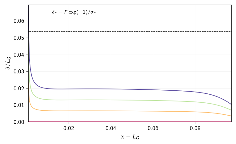
Let us just check the opening along the cohesive line at the end of the loading. Since we have tied the two surfaces of the crack together using a stiff penalty potential, we expect the opening to be very small much less than the critical opening displacement \(\delta_c\).
Figure 19.2: Opening along the cohesive line at different loading steps. The loading steps increase from as the color changes from red to blue. Dashed line indicates the critical opening displacement.
Phase 2: Dynamic Propagation
So we have our plate stretched out to near the critical load for crack propagation. Now we will let the crack propagate dynamically. To do so, we will use an explicit time integration scheme to solve the equations of motion including the inertial terms.
Since we want to make the crack propagate we will have to replace the penalty energy with a cohesive energy that allows for separation of the two surfaces once the critical traction is reached.
The total energy for a dynamic fracture problem is given by: \[E_{\text{total}} = T_{\text{kinetic}}(\dot{\boldsymbol{u}}) + \Psi_{\text{elastic}}(\boldsymbol{u}) + \Psi_{\text{fracture}}(\boldsymbol{u})\]
From the above equatiion, we have already defined the elastic strain energy \(\Psi_{\text{elastic}}\) in the previous section. We will now define the fracture energy \(\Psi_{\text{fracture}}\) and the kinetic energy \(E_{\text{kinetic}}\).
Use jax.jacrev to compute the internal force from the total energy defined above.
Note
Define below the function to compute the total energy\(\Psi(\boldsymbol{u})\) using elastic and fracture energies. The use jax.jacrev to compute the internal force from the total energy.
@jax.jitdef total_energy(u_flat: Array) ->float: u = u_flat.reshape(-1, n_dofs_per_node) elastic_strain_energy = total_strain_energy(u) cohesive_energy = total_cohesive_energy(u)return elastic_strain_energy + cohesive_energy# creating functions to compute the gradient andgradient = jax.jacrev(total_energy)
Deriving the Equation of Motion from Energy \(E\)
In our quasi-static simulations, we found the equilibrium state by minimizing the total potential energy \(\Psi(\boldsymbol{u})\).
In dynamics, we must account for the motion of the material. To do this, we introduce the Kinetic Energy, \(T\):
where \(\boldsymbol{m}\) is the mass vector and \(\dot{\boldsymbol{u}}\) is the velocity vector.
To derive the governing equations, we define the Lagrangian\(\mathcal{L}\) of the system, which is the difference between the kinetic energy and the potential energy:
Inertial Term: The derivative with respect to velocity gives momentum, and its time derivative gives the inertial force: \[\frac{d}{dt} \left( \frac{\partial T}{\partial \dot{\boldsymbol{u}}} \right) = \frac{d}{dt} (\mathbf{M} \dot{\boldsymbol{u}}) = \mathbf{M} \ddot{\boldsymbol{u}}\]
Internal Force Term: The derivative of the potential energy recovers our familiar internal and external forces: \[- \frac{\partial \mathcal{L}}{\partial \boldsymbol{u}} = \frac{\partial \Psi}{\partial \boldsymbol{u}} = \boldsymbol{f}_{\text{int}} - \boldsymbol{f}_{\text{ext}}\]
Combining these, we arrive at the dynamic equation of motion:
This is the equation we must solve at every time step. To solve the above equation, we will use an explicit time integration scheme based on the Newmark-\(\beta\) method (Central Difference).
Explicit time integration scheme
We present the explicit time integration scheme based on the Newmark-\(\beta\) method (Central Difference).
For this specific problem, we are transitioning from a quasi-static state. The boundary conditions for the dynamic phase are: * Displacement: Fixed at the final quasi-static value (\(\boldsymbol{u}_{\text{static}}\)) on the boundaries. * Velocity & Acceleration: Clamped to zero on the boundaries.
1. Predictor
First, we predict the state at \(n+1\) based on the current kinematic state.
\[
\dot{u}^{0}_{n+1} = \dot{u}_{n} + \Delta t \ddot{u}_{n}
\]
\[
\ddot{u}^{0}_{n+1} = \ddot{u}_{n}
\]
Apply Boundary Conditions (Displacement): At the fixed boundary DOFs, we must overwrite the prediction to maintain the clamped state: \[u^{0}_{n+1} |_{\text{bnd}} = u_{\text{static}} |_{\text{bnd}}\]
2. Solve
We calculate the acceleration update \(\delta \ddot{u}\) required to satisfy the equation of motion.
Apply Boundary Conditions (Residual): To ensure the boundaries do not accelerate, we force the residual to zero at those DOFs: \[\boldsymbol{r} |_{\text{bnd}} = 0\]
Apply Boundary Conditions (Velocity): As a final safety check to prevent numerical drift, we explicitly clamp the velocity and acceleration to zero at the boundaries: \[\dot{u}^{1}_{n+1} |_{\text{bnd}} = 0, \quad \ddot{u}^{1}_{n+1} |_{\text{bnd}} = 0\]
In order to correctly implement the explicit time integration scheme, we need two important things:
the mass vector \(\boldsymbol{m}\)
the critical time step \(\Delta t\) for stability.
Computing the mass vector \(\boldsymbol{m}\)
To compute the mass vector, we will use a lumped mass approach. In this approach, the mass associated with each node is computed by summing up the contributions from all elements connected to that node. The contribution from each element is computed based on the element’s volume and density. Below we define a function to compute the lumped mass vector mass_vector, \(\boldsymbol{m}\)
The dimension of the mass vector will be equal to the number of degrees of freedom in the system. Each entry in the mass vector corresponds to the mass associated with a specific degree of freedom (DOF) in the system.
rho =1025# kg/m^3@autovmap(u=1)def compute_area(u : Array) ->float:return u * rhodef total_area(u_flat): u = u_flat.reshape(-1, n_dofs_per_node) quad_values = op.eval(u) density = compute_area(quad_values)return jnp.sum(op.integrate(density))ones = jnp.ones(n_dofs)mass_vector = jax.jacrev(total_area)(ones)print(mass_vector)
The explicit time integration is conditionally stable. The critical time step is given by:
\[
\Delta t \leq \frac{h}{c}
\]
where \(h\) is the minimum element size and \(c\) is the wave speed.
The wave speed is given by:
\[
c = \sqrt{\frac{\mu + \lambda}{\rho}}
\]
where \(\mu\) and \(\lambda\) are the Lame parameters and \(\rho\) is the density.
The minimum element size is the radius of the inscribed circle of the element. Below we define a function to compute the radius of the inscribed circle of the element.
@autovmap(coords=2)def get_inscribed_circle_radius(coords): c1, c2, c3 = coords a = jnp.linalg.norm(c2 - c1) b = jnp.linalg.norm(c3 - c2) c = jnp.linalg.norm(c1 - c3) s = (a + b + c) /2 area = jnp.sqrt(s * (s - a) * (s - b) * (s - c))return area / s /2h_min = jnp.min(get_inscribed_circle_radius(coords[elements]))dt =0.5* h_min / (jnp.sqrt((2* mat.mu + mat.lmbda) / rho))print(f"critical time step: {dt}")
critical time step: 2.917544943000097e-06
Using the above two defined quantites, implement the explicit time integration scheme to simulate the dynamic propagation of the crack. The initial conditions are given by the static solution.
We will run the simulation for 4500 time steps. At every 100 time steps, we will store the following quantities:
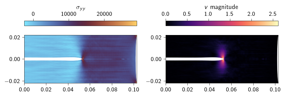
We can now plot the deformed configuration of the plate with the propagating crack. We will plot the deformed configuration at last time step to visualize the stresses in y-direction and the magnitude of the velocity field.
Figure 20.1: Snapshot of deformed configuration with crack propagation. Left figure shows the stress distribution, right figure shows the velocity magnitude.
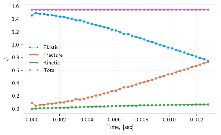
Energy conservation
We now plot the total energy of the system to check for energy conservation. The total energy is given by the sum of the kinetic energy, elastic strain energy, and the fracture energy. Since we ficed the displacement at the boundaries, the external work is zero, therefore the total energy should be constant.
What we should see is that while the total energy remains constant, there is an exchange between the kinetic energy, elastic strain energy, and the fracture energy as the crack propagates.
Figure 20.2: Energy curves for elastic, fracture and kinetic energies.
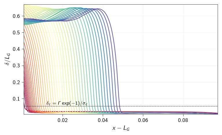
Crack tip opening
Now, let us see how crack tip opening \(\delta\) evolves as a function of time along the cohesive line looks like. We compute the jump \([\![\boldsymbol{u}]\!]\) vector at each quadrature point along the cohesive line. We use the line_op operator, defined earlier, to evaluate the jump at the quadrature points of the cohesive line. We will the use the jump values to compute the crack opening displacement (\(\delta\)) at each quadrature point along the cohesive line.
The quadrature points coordinates are also calculated using the line_op operator.
Figure 20.3: Opening along the cohesive line at different time steps. The time increases from red to blue.
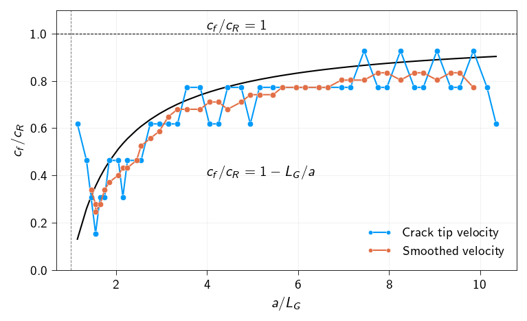
Crack Tip Velocity and the Speed Limit
Now we analyze the kinematics of the propagating crack. Unlike in the quasi-static case, the crack speed is governed by the full dynamic equation of motion, where the excess driving force (the difference between Energy Release Rate \(G\) and Fracture Energy \(\Gamma\)) is converted into Kinetic Energy.
However, a crack cannot accelerate indefinitely. Theoretical fracture mechanics predicts a universal speed limit: the Rayleigh wave speed (\(c_R\)), which is the speed at which surface waves travel in the material. As the crack tip approaches \(c_R\), the stress waves can no longer transport energy to the tip fast enough to sustain acceleration. The Rayleigh wave speed is approximately 92% of the shear wave speed \(c_s\) which is given by
\[
c_s = \sqrt{\frac{\mu}{\rho}}
\]
where \(\mu\) is the shear modulus and \(\rho\) is the density of the material.
In the plot below, we compare our numerical crack velocity against the theoretical prediction derived by Mott, which states that the velocity \(c_f\) evolves as
\[
c_\text{f}≈c_\text{R}(1−L_\text{G}/a),
\]
where \(a\) is the current crack length.
Note
For every 100th time step for which we stored the displacement \(\boldsymbol{u}\), compute the crack tip opening \(\delta\).
Determine the crack tip position as the location where the crack opening \(\delta\) reaches the critical opening \(\delta_c = \Gamma e^{-1}/\sigma_c\). Find the furthest point where \(\delta\) >= \(\delta_c\) from the original crack tip position. This gives the current crack tip position.
Compute the crack tip velocity as \[
c_\text{f} = \frac{da}{dt}
\]
by differentiating the crack tip position with respect to time. To reduce noise in the velocity data, apply a moving average filter with a window size of 5 time steps. - Finally, plot the normalized crack tip velocity \(c_f/c_R\) against the normalized crack length \(a/L_G\) and compare it with the theoretical prediction.
Code: Plot the crack tip velocity
def moving_average(data, window_size):"""Computes the moving average of a 1D array.""" window = jnp.ones(window_size) / window_size# mode='valid' returns an array of length N - K + 1return jnp.convolve(data, window, mode="valid")plt.style.use(STYLE_PATH)plt.figure(figsize=(5, 3), layout="constrained")ax = plt.axes()quadrature_points = line_op.eval(mesh.coords[bottom_cohesive_nodes]).squeeze()steps_to_plot = np.arange(0, len(u_per_step_dynamic))crack_tips = []crack_tip_velocity = []crack_times = []time_steps = np.arange(0, n_steps, 100) * dtdelta_c = cohesive_mat.Gamma * jnp.exp(-1) / cohesive_mat.sigma_cmycolor = plt.get_cmap("Spectral")(np.linspace(0, 1, len(steps_to_plot)))for i, c inzip(steps_to_plot, mycolor): jump_quad = line_op.eval( u_per_step_dynamic[i][top_cohesive_nodes]- u_per_step_dynamic[i][bottom_cohesive_nodes] ).squeeze() opening_quadrature = compute_opening(jump_quad) idx = np.argwhere(opening_quadrature >1.0* delta_c)[-1][0] crack_tip = quadrature_points[idx, 0] crack_tips.append(crack_tip) crack_times.append(time_steps[i])crack_tips = jnp.array(crack_tips).flatten()crack_times = jnp.array(crack_times).flatten()raw_velocity = np.gradient(crack_tips, crack_times)window_size =5iflen(raw_velocity) > window_size: smooth_velocity = moving_average(raw_velocity, window_size)# Because 'valid' convolution shortens the array, we need to trim# the x-axis (crack_tips) to match the new length.# We trim from the start/end to align the centers. trim_start = (window_size -1) //2 trim_end = trim_start +len(smooth_velocity) tips_for_plotting = crack_tips[trim_start:trim_end]else:# Fallback if not enough data points smooth_velocity = raw_velocity tips_for_plotting = crack_tipsc_shear = jnp.sqrt(mu / rho)c_rayleigh =0.92* c_shearax.plot(crack_tips / L_G, 1- L_G / crack_tips, color="black")ax.plot( crack_tips / L_G, raw_velocity / c_rayleigh,"o-", label="Crack tip velocity",)ax.plot( tips_for_plotting / L_G, smooth_velocity / c_rayleigh,"o-", label="Smoothed velocity",)ax.axhline(1.0, color="black", linewidth=0.5, ls="--")ax.text(4, 0.4, r"$c_f/c_R = 1- L_G/a$", color="black", fontsize=10)ax.text(4, 1.02, r"$c_f/c_R = 1$", color="black", fontsize=10)ax.axvline(1.0, color="grey", linewidth=0.5, ls="--")ax.set_xlabel(r"$a/L_G$")ax.set_ylabel(r"$c_f/c_R$")ax.grid(True)ax.legend(frameon=False)ax.set_ylim(top=1.1, bottom=0.0)plt.show()
Figure 20.4: Crack tip velocity as a function of crack length.