In this exercise, we will solve a linear elastic problem of a plate with a through crack. Using LEFM (Linear Elastic Fracture Mechanics) theory, we will analyze if a crack will nucleate under applied displacements. We will use the concept of energy release rate \(G\) and fracture energy density \(\Gamma\) to analyze the stability of the crack.
The plate will be subjected to a Mode I loading by applying a displacement on the top and bottom edges of the plate in the \(y\)-direction. The total potential energy of the system is given by:
\[
\Psi = \Psi_\text{e}
\]
where \(\Psi_\text{e}\) is the elastic strain energy of the system.
In this class activity, we do not numerically simulate the crack propagation. Instead, we will use the concept of energy release rate \(G\) and fracture energy density \(\Gamma\) to analyze if the crack will nucleate under the applied displacement (see Fundamentals of Fracture Mechanics for more details). The energy release rate \(G\) will be computed in two steps:
We solve the linear elastic problem for a given crack length \(a\) and applied displacement \(u\). We compute the total potential energy \(\Psi (a)\).
We generate a new mesh with a larger crack length \(a + \Delta a\) and solve the linear elastic problem again for the same applied displacement \(u\). We compute the total potential energy \(\Psi (a + \Delta a)\).
The energy release rate \(G\) is then computed as:
\[
G = - \frac{\text{d} \Psi}{\text{d} a} \approx - \big(\frac{\Psi (a + \Delta a) - \Psi (a)}{\Delta a}\big)
\]
We then compare the energy release rate \(G\) with the fracture energy density \(\Gamma\) to determine if the crack will nucleate.
Furthermore, we will test two different plate sizes and crack lengths to see how the energy release rate \(G\) depends on the global geometry of the plate and controls the nucleation of the crack.
Plate 1: \(2L=3.2\), \(H=0.32\), \(2a=0.16\)
Plate 2: \(2L=0.64\), \(H=0.056\), \(2a=0.16\)
where \(2a\) is the crack length. Instead of modelling the entire plate, we will model only half of the plate with a symmetry boundary condition on the mid-plane.
We will first setup our numerical framework to solve the linear elastic problem for plate 1 for crack length \(a\) and then usethe same framework to solve the linear elastic problem for plate 2 for crack length \(a\) and compute the energy release rate \(G\) for both the plates.
Model setup
As mentioned earlier, we will model only half of the plate with a symmetry boundary condition on the mid-plane. We provide a function generate_cracked_plate_mesh to generate the mesh for the a half plate with given dimensions and a pre-crack of length \(a\) from the left edge.
Function to generate a mesh with a pre-crack
def get_elements_on_curve(mesh, curve_func, tol=1e-3): coords = mesh.coords elements_2d = mesh.elements# Efficiently find all nodes on the curve using jax.vmap on_curve_mask = jax.vmap(lambda c: curve_func(c, tol))(coords) elements_1d = []# Iterate through all 2D elements to find edges on the curvefor tri in elements_2d:# Define the three edges of the triangle edges = [(tri[0], tri[1]), (tri[1], tri[2]), (tri[2], tri[0])]for n_a, n_b in edges:# If both nodes of an edge are on the curve, add it to the setif on_curve_mask[n_a] and on_curve_mask[n_b]:# Sort to store canonical representation, e.g., (1, 2) not (2, 1) elements_1d.append(tuple(sorted((n_a, n_b))))ifnot elements_1d:return jnp.array([], dtype=int)return jnp.array(elements_1d)def generate_cracked_plate_mesh( length: float, height: float, crack_tip_coords: tuple[float, float], mesh_size_crack: float, mesh_size_far: float, refine_dist_crack: float, output_filename: str="../meshes/lefm.msh"):""" Generates a 2D mesh using the Gmsh Python API based on the provided .geo script. Args: length (float): Total length 'L' of the domain. height (float): Total height 'H' of the domain. lc (float): Characteristic length 'l' for the initial point. min_elem (float): Minimum element size for the refinement box. output_filename (str): Name of the output mesh file (e.g., 'model.msh'). """ gmsh.initialize() gmsh.model.add("refined_plate")# --- Use OpenCASCADE geometry kernel ---#gmsh.model.setFactory("OpenCASCADE")# --- Define script parameters --- h2 =1.0 epsilon =1e-5 depth =0.0# --- Define geometry points ---# The last argument is the prescribed mesh size at that point. p1 = gmsh.model.geo.addPoint(0, epsilon, -depth /2) p2 = gmsh.model.geo.addPoint(crack_tip_coords[0], crack_tip_coords[1], -depth /2) p3 = gmsh.model.geo.addPoint(0, -epsilon, -depth /2) p4 = gmsh.model.geo.addPoint(0, -height /2, -depth /2) p5 = gmsh.model.geo.addPoint(length, -height /2, -depth /2) p6 = gmsh.model.geo.addPoint(length, height /2, -depth /2) p7 = gmsh.model.geo.addPoint(0, height /2, -depth /2)# --- Define lines connecting the points --- l1 = gmsh.model.geo.addLine(p1, p2) l2 = gmsh.model.geo.addLine(p2, p3) l3 = gmsh.model.geo.addLine(p3, p4) l4 = gmsh.model.geo.addLine(p4, p5) l5 = gmsh.model.geo.addLine(p5, p6) l6 = gmsh.model.geo.addLine(p6, p7) l7 = gmsh.model.geo.addLine(p7, p1)# --- Define curve loops and surfaces ---# A negative tag in a loop reverses the line's direction. loop1 = gmsh.model.geo.addCurveLoop([l1, l2, l3, l4, l5, l6, l7]) surface1 = gmsh.model.geo.addPlaneSurface([loop1])#crack_tip_p = gmsh.model.geo.addPoint(crack_tip_coords[0], crack_tip_coords[1], 0)# Synchronize the CAD kernel with the Gmsh model gmsh.model.geo.synchronize()# --- Define Physical Groups ---# Physical groups are used to identify boundaries and domains.# Physical Line(2) = {{2}}; gmsh.model.addPhysicalGroup(1, [loop1], 2) # dim=1 for lines# Physical Surface(1) = {{1, 2}}; gmsh.model.addPhysicalGroup(2, [surface1], 1) # dim=2 for surfaces# --- Define Mesh Refinement Field --- dist_field_crack = gmsh.model.mesh.field.add("Distance", 1) gmsh.model.mesh.field.setNumbers(dist_field_crack, "PointsList", [p2]) thresh_field_crack = gmsh.model.mesh.field.add("Threshold", 2) gmsh.model.mesh.field.setNumber(thresh_field_crack, "InField", dist_field_crack) gmsh.model.mesh.field.setNumber(thresh_field_crack, "SizeMin", mesh_size_crack) gmsh.model.mesh.field.setNumber(thresh_field_crack, "SizeMax", mesh_size_far) gmsh.model.mesh.field.setNumber(thresh_field_crack, "DistMin", refine_dist_crack) gmsh.model.mesh.field.setNumber( thresh_field_crack, "DistMax", refine_dist_crack *2 )# Set this field as the background field, which Gmsh uses to drive mesh generation. gmsh.model.mesh.field.setAsBackgroundMesh(thresh_field_crack)# --- Set global mesh options ---# These options prevent Gmsh from overriding the background field. gmsh.option.setNumber("Mesh.CharacteristicLengthFromPoints", 0) gmsh.option.setNumber("Mesh.CharacteristicLengthFromCurvature", 0) gmsh.option.setNumber("Mesh.CharacteristicLengthExtendFromBoundary", 0)# --- Generate the 2D mesh --- gmsh.model.mesh.generate(2)# --- Save the mesh and optionally launch the GUI --- gmsh.write(output_filename)print(f"Mesh saved to '{output_filename}'") gmsh.finalize() _mesh = meshio.read(output_filename) mesh = Mesh( coords=_mesh.points[:, :2], elements=_mesh.cells_dict["triangle"], )return mesh
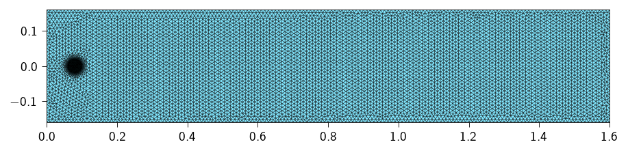
For plate 1, since we model only half of the plate, we start with plate of dimension \(L=1.6\) and \(H=0.32\) with a crack of length \(a=0.08\) from the left edge.
We refine the mesh near the crack tip to capture the stress field near the crack tip accurately. We use a mesh size of \(5 \times 10^{-4}\) for the crack tip region and \(1 \times 10^{-2}\) for the rest of the plate. We use a distance of \(0.02\) to control the size of the elements near the crack tip.
The parameters are passed to the generate_cracked_plate_mesh function to generate the mesh
Figure 15.1: Visualization of the mesh. We refine the mesh near the crack tip to capture the stress field near the crack tip accurately.
Defining material parameters
Let us define the material parameters mainly the shear modulus and the first Lamé parameter. The Youngs modulus and the Poisson’s ratio are related for the material are:
\[
E = 10^{6} ~\text{N/m}^2, \quad \nu = 0.3
\]
From the above, we can compute the shear modulus and the first Lamé parameter as:
tri = element.Tri3()op = Operator(mesh, tri)@autovmap(grad_u=2)def compute_strain(grad_u: Array) -> Array:"""Compute the strain tensor from the gradient of the displacement."""return0.5* (grad_u + grad_u.swapaxes(-1, -2))@autovmap(eps=2)def compute_stress(eps: Array, mu: float, lmbda: float) -> Array:"""Compute the stress tensor from the strain tensor.""" I = jnp.eye(2)return2* mu * eps + lmbda * jnp.trace(eps) * I@autovmap(grad_u=2)def strain_energy(grad_u: Array, mu: float, lmbda: float) -> Array:"""Compute the strain energy density.""" eps = compute_strain(grad_u) sig = compute_stress(eps, mu, lmbda)return0.5* jnp.einsum("ij,ij->", sig, eps)@jax.jitdef total_energy(u_flat): u = u_flat.reshape(-1, n_dofs_per_node) u_grad = op.grad(u) energy_density = strain_energy(u_grad, mat.mu, mat.lmbda)return op.integrate(energy_density)
Computing the internal forces and the stiffness matrix
For this exercise, we will like to use the sparse solver, given the large number of degrees of freedom. We will use the sparse module to compute the sparsity pattern and then use the sparse.jacfwd to compute the Jacobian of the internal forces.
We apply a prestrain of \(\varepsilon_{\infty} = 0.01\) to the top and bottom edges of the plate. The prestrain is applied in the direction of the \(y\)-axis. The prestrain is applied as displacement boundary conditions both on the top and the botttom nodes. \[
u_y (y=y_\text{max}) = \varepsilon_{\infty} L_y / 2.
\]\[
u_y (y=y_\text{min}) = -\varepsilon_{\infty} L_y / 2
\]
where \(L_y\) is the height of the plate.
We also fix the displacement in the \(x\)-direction on the top and bottom nodes i.e.
\[
u_x (y=y_\text{max}) = 0
\]
and
\[
u_x (y=y_\text{min}) = 0
\]
Due to symmetry, the left edge of the plate is fixed in the \(x\)-direction i.e.
We apply boundary conditions using the lifting approach. To apply the lifting to a sparse stiffness matrix, we need the indices corresponding the rows and columns that are fixed (to be set to zero) and the indices of the diagonal elements that are set to one.
Below use the sparse.get_bc_indices to get the indices (row, col) where we set the stiffness entries to zero and the indices of the diagonal elements that are set to one.
We will use the Newton’s method to solve the problem. Remember we use the lifting approach to apply the boundary conditions, therefore, we need to modify the stiffness matrix and the residual vector to account for the boundary conditions. See Sparse solvers for more details on how to use the lifting approach within a Newton solver.
Implement the newton_sparse_solver function to solve the problem using the Newton’s method.
Newton-Raphson solver
import scipy.sparse as spdef newton_scipy_solver( u, fext, gradient, hessian_sparse, fixed_dofs, zero_indices, one_indices,): fint = gradient(u) K_sparse = hessian_sparse(u) indices = K_sparse.indices du = jnp.zeros_like(u) iiter =0 norm_res =1.0 tol =1e-8 max_iter =110while norm_res > tol and iiter < max_iter: residual = fext - fint residual = residual.at[fixed_dofs].set(0) K_data_lifted = K_sparse.data.at[zero_indices].set(0) K_data_lifted = K_data_lifted.at[one_indices].set(1) K_csr = sp.csr_matrix((K_data_lifted, (indices[:, 0], indices[:, 1]))) du = sp.linalg.spsolve(K_csr, residual) u = u.at[:].add(du) fint = gradient(u) K_sparse = hessian_sparse(u) residual = fext - fint residual = residual.at[fixed_dofs].set(0) norm_res = jnp.linalg.norm(residual)print(f" Residual: {norm_res:.2e}") iiter +=1return u, norm_res
Implementing the Incremental Loading Loop
Now that we have the mesh, the energy functions, and the newton_sparse_solver, it’s time to set up the main simulation loop. We will apply the displacement in small increments and solve for equilibrium at each step.
We divide the total displacement into 5 steps and solve the system of equations for each step.
Hint
The loop will look like this:
for step inrange(n_steps):print(f"Step {step+1}/{n_steps}")# ... Your code for each step will go inside this loop ...
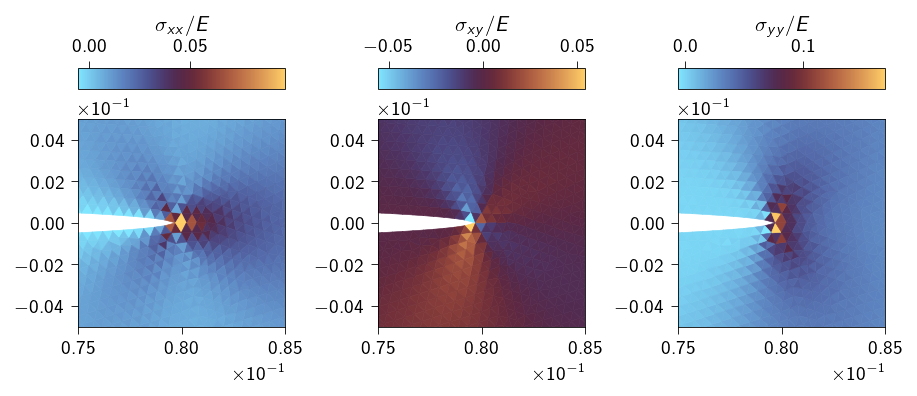
We plot the stress field near the crack tip. We can see that the stress field is concentrated near the crack tip and the stress field is highest at the crack tip.
Computing crack nucleation and prediction of crack growth
Now lets compute the energy release rate \(G\) using the virtual crack extension method. We will extended the crack by a small amount and compute the energy released due to the extension.
We will use the following formula to compute the energy release rate:
where \(\Psi_0\) and \(\Psi_1\) are the potential energies before and after the crack extension, respectively, and \(a_0\) and \(a_1\) are the crack lengths before and after the extension, respectively.
We will compute the energy release rate for two different plate sizes (Plate 1 and Plate 2) with same pre-crack length of \(2a=0.16\). Both the plates are made of the same material with the following properties:
\(E=10^6 ~\text{N/m}^2\)
\(\nu=0.3\)
\(\Gamma = 22.4~ \text{ J/m}^2\)
For both the plate configuration, we would like to answer the following questions:
For what applied displacement, the crack will nucleate?
Upon nucleation, under same applied displacement, will the crack grow in the plate or not?
The two different plate configurations considered in this activity. The plate on the left is a wide plate and the plate on the right is a thin strip.
To ensure good enough accuracy, we need to use a mesh size that is small enough to resolve the crack tip. We will use a mesh size of \(5\times 10^{-4}\) for the crack tip and \(10^{-2}\) for the far field while calling the function generate_cracked_plate_mesh.
length =1.6height =0.32mesh_size_crack =5e-4mesh_size_far =1e-2crack_length = ... # choose a crack length from the list of crack lengthsrefine_dist_crack =0.02params = {"length": length,"height": height,"crack_tip_coords": (crack_length, 0.0),"mesh_size_crack": 5e-4, "mesh_size_far": 1e-2, "refine_dist_crack": refine_dist_crack,}mesh = generate_cracked_plate_mesh(**params)
Note
The workflow for the simulation will be as follows:
Assume a applied displacement on the top and the bottom nodes.
For crack length \(a_0\), compute the energy release rate \(G\). Remember you will have to do two simulations to compute the energy release rate. One at \(a_0\) and one at \(a_1\). The applied displacement will be same for both the simulations.
Compute the energy release rate \(G\) using the formula \[G(a) = - \big(\frac{\Psi(a + \Delta a) - \Psi(a)}{\Delta a}\big)\]
If \(G(a)\) is greater than the fracture energy \(\Gamma\), then the crack will nucleate.
This applied displacement is the displacement that causes the crack to nucleate.
Now run the simulations for different crack lengths. Compute the elastic strain energy for each crack length and use it to compute the energy release rate \(G\) for each crack length.
Remember the applied displacement on the top and the bottom nodes is same for all the crack lengths which is equal to the displacement that causes the crack to nucleate.
🐍 Download source code
In order to perform the above computations for different plate sizes and crack lengths, we will wrap the code in a function called solve_lefm. Click below to download the script that contains the function solve_lefm used below.
To ensure good enough accuracy, we need to use a mesh size that is small enough to resolve the crack tip. We will use a mesh size of \(5\times 10^{-4}\) for the crack tip and \(10^{-2}\) for the far field while calling the function generate_cracked_plate_mesh.
length =0.32height =0.056crack_length = ... # choose a crack length from the list of crack lengthsrefine_dist_crack =0.02params = {"length": length,"height": height,"crack_tip_coords": (crack_length, 0.0),"mesh_size_crack": 5e-4, "mesh_size_far": 1e-2, "refine_dist_crack": refine_dist_crack,}mesh = generate_cracked_plate_mesh(**params)
Note
The workflow for the simulation will be as follows:
Assume a applied displacement on the top and the bottom nodes.
For crack length \(a_0\), compute the energy release rate \(G\). Remember you will have to do two simulations to compute the energy release rate. One at \(a_0\) and one at \(a_1\). The applied displacement will be same for both the simulations.
Compute the energy release rate \(G\) using the formula \[G(a) = - \big(\frac{\Psi(a + \Delta a) - \Psi(a)}{\Delta a}\big)\]
If \(G(a)\) is greater than the fracture energy \(\Gamma\), then the crack will nucleate.
This applied displacement is the displacement that causes the crack to nucleate.
Now run the simulations for different crack lengths. Compute the elastic strain energy for each crack length and use it to compute the energy release rate \(G\) for each crack length.
Remember the applied displacement on the top and the bottom nodes is same for all the crack lengths which is equal to the displacement that causes the crack to nucleate.
The energy release rate \(G\) for Plate 2 at different crack lengths is:
plate_2_Gs =-np.diff(plate_2_potential_energies) / np.diff(crack_lengths)print("The energy release rate G for Plate 2: ", plate_2_Gs)
The energy release rate G for Plate 2: [22.6267366 22.6287959 22.61852869 22.5886829 22.60493786 22.53718251]
Note
Question 2: For what applied displacement, the crack will nucleate in Plate 2? Is it different from the applied displacement for Plate 1? If both the plates are made of same material, why is the crack nucleation displacement different?
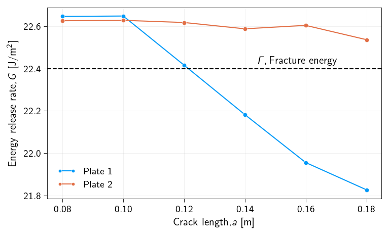
Now we plot the energy release rate \(G(a)\) for both the plates. We also plot the critical energy release rate \(\Gamma\) for both the plates. Use this information to answer the questions whether under the applied displacement (that causes the crack to nucleate) will the crack grow in the two plates or not for the give range of ctack extensions.
Figure 15.3: Energy release rate G for both the plates. A comparison with the fracture energy is also shown.
Note
Question 3: For which plate the crack will grow if we keep the applied displacement that causes the crack to nucleate for each plate respectively? Explain your answer.