In this exercise, we apply the concepts learned in the In-class activity: Cohesive zone modelling to simulate crack propagation in a plate under quasistatic loading. We will use a 2D plate with a pre-crack of length slightly larger than the Griffith fracture length loaded under Mode I loading.
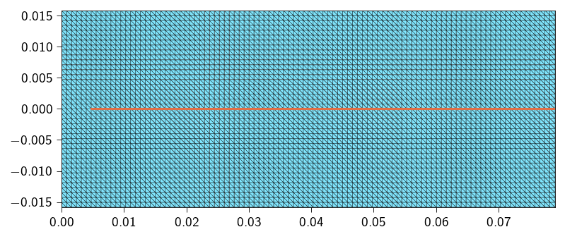
An animation of the crack propagation is shown below. The stress value shown is \(\sigma_{yy}\).
We will assume that the crack propagates in a straight line in the \(x\)-direction which is known. This assumption is valid enough for this exercise as the loading is in Mode I. Furthermore, becuase of this assumption we know the \(\Gamma_\text{coh}\) and we can use the line elements to tie the two blocks of the plate together using Traction-Separation law. Therefore, for the plate the total potential energy is given by:
the effect of applied displacement on the crack propagation
how the energies are distributed as the crack propagates,
how to determine the crack opening and henceforth the crack tip location of a propagating crack.
Code: Importing the essential libraries
import jaxjax.config.update("jax_enable_x64", True) # use double-precisionjax.config.update("jax_persistent_cache_min_compile_time_secs", 0)jax.config.update("jax_platforms", "cpu")import jax.numpy as jnpfrom jax import Arrayfrom tatva import Mesh, Operator, elementfrom tatva.plotting import ( STYLE_PATH, colors, plot_element_values,)from jax_autovmap import autovmapfrom typing import Callable, Optional, Tupleimport numpy as npimport matplotlib.pyplot as plt
Model setup
For our model setup, we consider a plate with a pre-crack of length \(a_0\) subjected to tensile loading on the top and bottom surfaces. The plate is subjected to a prestrain of \(\varepsilon^0 = 0.1\). In order to ensure that for this applied displacement, the crack \(a_0\) nucleates and propagates, we make use of the the energy balance criteria i._e
\[
G = \Gamma = \frac{K_I^2}{E'}
\]
where \(G\) is the energy release rate, \(\Gamma\) is the fracture energy, \(K_I\) is the stress intensity factor and \(E'\) is the effective elastic modulus. For an infinite plate with a pre-crack of length \(a\), the stress intensity factor is given by:
\[
K_I = \sigma_\infty \sqrt{\pi a}
\]
Equating the two relations, we get
\[
a = \dfrac{1}{\pi}\frac{\Gamma E } {(1-\nu^2 )\sigma_\infty^2}
\] The above expression tells that for an infinite plate with the applied stress \(\sigma_\infty\) is inversely proportional to the critical crack length \(a\). This means that if we have a small pre-crack, the applied stress \(\sigma_\infty\) will be large to make it nucleate when compared to a plate with a larger pre-crack. This gives the minimum crack length \(a\) for which the crack will nucleate and propagate at the applied stress \(\sigma_\infty\).
In this notebook, we use \(L_G\) to denote the critical crack length
\[
L_G = a
\]
We will use the above relation to determine the critical crack length for our model setup. We will use the following material parameters:
and the applied stress \(\sigma_\infty = \varepsilon^0 /E_\text{eff}\) where \(E_\text{eff}\) is the effective Young’s modulus and \(E_\text{eff} = E/(1-\nu^2)\) is the effective Young’s modulus.
prestrain =0.1nu =0.35E =106e3# N/m^2lmbda = nu * E / ((1+ nu) * (1-2* nu))mu = E / (2* (1+ nu))Gamma =15# J/m^2sigma_c =20e3# N/m^2print(f"mu: {mu} N/m^2")print(f"lmbda: {lmbda} N/m^2")sigma_inf = prestrain * E / (1- nu**2)L_G =2* mu * Gamma / (jnp.pi * (1- nu) * sigma_inf**2)print(f"L_G: {L_G} m")
mu: 39259.259259259255 N/m^2
lmbda: 91604.93827160491 N/m^2
L_G: 0.003952597997069948 m
Using the above dimensions, we define a domain of length \(20\times L_G\) and height \(8\times L_G\). The plate has a pre-crack of length slightly larger than the Griffith fracture length \(L_G\).
For this exercise, we will use a pre-crack length of \(1.0\times L_G\). We use triangular elements to discretize the domain.
Code: Functions to generate the mesh
def generate_mesh_with_line_elements( nx: int, ny: int, lxs: Tuple[float, float], lys: Tuple[float, float], curve_func: Optional[Callable[[Array, float], bool]] =None, tol: float=1e-6,) -> Tuple[Array, Array, Optional[Array]]:""" Generates a 2D triangular mesh for a rectangle and optionally extracts 1D line elements along a specified curve. Args: nx: Number of elements along the x-direction. ny: Number of elements along the y-direction. lxs: Tuple of the x-coordinates of the left and right edges of the rectangle. lys: Tuple of the y-coordinates of the bottom and top edges of the rectangle. curve_func: An optional callable that takes a coordinate array [x, y] and a tolerance, returning True if the point is on the curve. tol: Tolerance for floating-point comparisons. Returns: A tuple containing: - coords (jnp.ndarray): Nodal coordinates, shape (num_nodes, 2). - elements_2d (jnp.ndarray): 2D triangular element connectivity. - elements_1d (jnp.ndarray | None): 1D line element connectivity, or None. """ x = jnp.linspace(lxs[0], lxs[1], nx +1) y = jnp.linspace(lys[0], lys[1], ny +1) xv, yv = jnp.meshgrid(x, y, indexing="ij") coords = jnp.stack([xv.ravel(), yv.ravel()], axis=-1)def node_id(i, j):return i * (ny +1) + j elements_2d = []for i inrange(nx):for j inrange(ny): n0 = node_id(i, j) n1 = node_id(i +1, j) n2 = node_id(i, j +1) n3 = node_id(i +1, j +1)#elements_2d.append([n0, n1, n3])#elements_2d.append([n0, n3, n2]) elements_2d.append([n0, n1, n2]) elements_2d.append([n1, n3, n2]) elements_2d = jnp.array(elements_2d)# Extract 1D elements if a curve function is provided ---if curve_func isNone:return coords, elements_2d, None# Efficiently find all nodes on the curve using jax.vmap on_curve_mask = jax.vmap(lambda c: curve_func(c, tol))(coords) elements_1d = []# Iterate through all 2D elements to find edges on the curvefor tri in elements_2d:# Define the three edges of the triangle edges = [(tri[0], tri[1]), (tri[1], tri[2]), (tri[2], tri[0])]for n_a, n_b in edges:# If both nodes of an edge are on the curve, add it to the setif on_curve_mask[n_a] and on_curve_mask[n_b]:# Sort to store canonical representation, e.g., (1, 2) not (2, 1) elements_1d.append(tuple(sorted((n_a, n_b))))ifnot elements_1d:return coords, elements_2d, jnp.array([], dtype=int)return coords, elements_2d, jnp.unique(jnp.array(elements_1d), axis=0)
Nx =100# Number of elements in XNy =20# Number of elements in YLx =20* L_G # Length in XLy =8* L_G # Length in Ycrack_length =1.0* L_G# function identifies nodes on the cohesive line at y = 0. and x > 2.0def cohesive_line(coord: Array, tol: float) ->bool:return jnp.logical_and( jnp.isclose(coord[1], 0.0, atol=tol), coord[0] > crack_length )upper_coords, upper_elements_2d, top_interface_elements = generate_mesh_with_line_elements( nx=Nx, ny=Ny, lxs=(0, Lx), lys=(0, Ly/2), curve_func=cohesive_line)lower_coords, lower_elements_2d, bottom_interface_elements = generate_mesh_with_line_elements( nx=Nx, ny=Ny, lxs=(0, Lx), lys=(-Ly/2, 0), curve_func=cohesive_line)coords = jnp.vstack((upper_coords, lower_coords))elements = jnp.vstack((upper_elements_2d, lower_elements_2d + upper_coords.shape[0]))mesh = Mesh(coords, elements)n_nodes = mesh.coords.shape[0]n_dofs_per_node =2n_dofs = n_dofs_per_node * n_nodesbottom_interface_elements = bottom_interface_elements + upper_coords.shape[0]
\(\boldsymbol{\delta}(\boldsymbol{u}) = f([\![\boldsymbol{u}]\!])\) is the displacement jump across the interface.
\(\psi(\boldsymbol{\delta})\) is the cohesive potential, which defines the energy-separation relationship.
Defining the operator for line integration
We will begin by defining the operator for line integration similar to Operator that we have used for the triangular elements. To do so, we will have to first define the line elements along the potential fracture surface. We will use the Line2 element to define the line elements. This element has 2 nodes. Below, we use the function extract_interface_mesh to generate the mesh that consists of the line elements along the potential fracture surface. Since are two blocks have two surfaces along which the fracture can propagate (upper and lower), we can use any one of the two surfaces to define the cohesive zone. Here, we use the lower surface. We will define a new mesh that contains the line elements from one of the two interfaces. Since the two interfaces are discretized using the same number of elements, and occupy the same spatial domain, we can use any one of the two to perform the integration.
Code: Generate the interface mesh
def extract_interface_mesh(mesh, line_elements):"""Generate a mesh for the interface between two materials."""# --- Interface mesh --- line_element_nodes = jnp.unique(line_elements.flatten()) interface_coords = mesh.coords[line_element_nodes] interface_elements = jnp.array( [[index, index +1] for index inrange(len(line_elements))] ) interface_mesh = Mesh(interface_coords, interface_elements)return interface_mesh
Use the above defined function extract_interface_mesh to generate the interface mesh and then define the line_op operator.
where \(\delta_c = \frac{\Gamma e^{-1}}{\sigma_c}\) is the critical separation, \(\Gamma\) is the fracture energy, \(\sigma_c\) is the critical stress, and \(e\) is the base of the natural logarithm.
where \(\boldsymbol{t}\) is the tangential direction (which for this problem is the \(x\)-direction) and \(\boldsymbol{n}\) is the normal direction to the cohesive interface (which for this problem is the \(y\)-direction).
Note
If you notice, the potential is also defined for \(\delta < 0\). When \(\delta < 0\), it means that the two surfaces are actually penetrating each other. In this case, we use a penalty like term to penalize the interpenetration. This is exactly similar to the penalty method used in the contact mechanics.
Remember at this point we do not introduce the irreversibility in the cohesive potential. This will be done in the next lectures.
In order to compute the \(\psi(\delta)\) for an exponential traction-separation law we need to perform the following steps:
Compute the opening \(\delta\) along the cohesive interface is defined as:
where \(\boldsymbol{t}\) is the tangential direction (which for this problem is the \(x\)-direction) and \(\boldsymbol{n}\) is the normal direction to the cohesive interface (which for this problem is the \(y\)-direction).
Compute the cohesive energy density \(\psi(\delta)\) using the exponential traction-separation potential.
The function to compute the opening of the cohesive element will look like this:
@autovmap(jump=1)def compute_opening(jump: jnp.ndarray) ->float:""" Compute the opening of the cohesive element. Args: jump: The jump in the displacement field, which is the difference between the displacement of the upper and lower bodies across the crack. Returns: The opening of the cohesive element. """ opening = ... # TODO: Compute the opening of the cohesive elementreturn opening
The function to compute the cohesive energy density will look like this:
@autovmap(jump=1)def exponential_cohesive_energy( jump: jnp.ndarray, Gamma: float, sigma_c: float, penalty: float, delta_threshold: float=0.0,) ->float:""" Compute the cohesive energy for a given jump. Args: jump: The jump in the displacement field. Gamma: Fracture energy of the material. sigma_c: The critical strength of the material. penalty: The penalty parameter for penalizing the interpenetration. """ delta = ... # TODO: Compute the opening of the cohesive element ... # TODO: check if delta is greater than the threshold ... # TODO: if delta is greater than the threshold, compute the cohesive energy density using the exponential traction-separation potential ... # TODO: if delta is less than the threshold, return 0.5 * penalty * delta**2return cohesive_energy_density
In order to check if the delta is greater than the threshold, use the jax.lax.cond function.
Moreover, use the below defined safe_sqrt function to compute the square root of the delta. We redefine the square root function because default square root function is non-differentiable at zero because of the limit definition of the square root. Here we use the jnp.where function to return zero when the input is less than or equal to zero. This makes the square root function differentiable at zero.
@jax.jitdef safe_sqrt(x):return jnp.sqrt(jnp.where(x >0.0, x, 0.0))@autovmap(jump=1)def compute_opening(jump: Array) ->float:""" Compute the opening of the cohesive element. Args: jump: The jump in the displacement field. Returns: The opening of the cohesive element. """ opening = safe_sqrt(jump[0] **2+ jump[1] **2)return opening@autovmap(jump=1)def exponential_cohesive_energy( jump: Array, Gamma: float, sigma_c: float, penalty: float, delta_threshold: float=1e-8,) ->float:""" Compute the cohesive energy for a given jump. Args: jump: The jump in the displacement field. Gamma: Fracture energy of the material. sigma_c: The critical strength of the material. penalty: The penalty parameter for penalizing the interpenetration. delta_threshold: The threshold for the delta parameter. Returns: The cohesive energy. """ delta = compute_opening(jump) delta_c = (Gamma * jnp.exp(-1)) / sigma_cdef true_fun(delta):return Gamma * (1- (1+ (delta / delta_c)) * (jnp.exp(-delta / delta_c)))def false_fun(delta):return0.5* penalty * delta**2return jax.lax.cond(delta > delta_threshold, true_fun, false_fun, delta)
Now use the above defined function and the line_op operator to compute the fracture energy. The fracture energy is then given by:
We now locate the dofs in the two domains to apply boundary conditions. We load the domain under Model I loading where both the top and bottom surfaces are loaded along the \(y\)-direction only. Furthermore, we assume symmetry about the \(x\)-axis at the left edge of the domain. Under symmetry, the domain represents a thorough crack in the middle of the domain. So the boundary conditions are:
\(u_x = 0\) on the left edge
\(u_y = -H\varepsilon_0/2\) on the bottom edge
\(u_y = H\varepsilon_0/2\) on the top edge
\(u_x = 0\) on the top and bottom edges
where \(H\) is the height of the domain and \(\varepsilon_0\) is the applied prestrain.
Now, we define a few functions to implement the matrix-free solvers. We will use the conjugate gradient method to solve the linear system of equations. The Dirichlet boundary conditions are applied using projection method. As we use the matrix-free solver, we need to define the gradient of the total potential energy, which is also the residual function.
Below define the function to compute the \(\boldsymbol{f}_{int}\) using jax.jacrev and then use this function to compute the Jacobian-vector product using jax.jvp. Remember to apply the Projection approach to enforce the Dirichlet boundary conditions.
# creating functions to compute the gradient andgradient = jax.jacrev(total_energy)# create a function to compute the JVP product@jax.jitdef compute_tangent(du, u_prev): du_projected = du.at[fixed_dofs].set(0) tangent = jax.jvp(gradient, (u_prev,), (du_projected,))[1] tangent = tangent.at[fixed_dofs].set(0)return tangent
Code: Functions to implement the conjugate gradient method and Netwon-Raphson method
from functools import partialimport equinox as eqx#@partial(jax.jit, static_argnames=["A", "atol", "max_iter"])@eqx.filter_jitdef conjugate_gradient(A, b, atol=1e-8, max_iter=100): iiter =0def body_fun(state): b, p, r, rsold, x, iiter = state Ap = A(p) alpha = rsold / jnp.vdot(p, Ap) x = x + jnp.dot(alpha, p) r = r - jnp.dot(alpha, Ap) rsnew = jnp.vdot(r, r) p = r + (rsnew / rsold) * p rsold = rsnew iiter = iiter +1return (b, p, r, rsold, x, iiter)def cond_fun(state): b, p, r, rsold, x, iiter = statereturn jnp.logical_and(jnp.sqrt(rsold) > atol, iiter < max_iter) x = jnp.full_like(b, fill_value=0.0) r = b - A(x) p = r rsold = jnp.vdot(r, p) b, p, r, rsold, x, iiter = jax.lax.while_loop( cond_fun, body_fun, (b, p, r, rsold, x, iiter) )return x, iiterdef newton_krylov_solver( u, fext, gradient, fixed_dofs,): fint = gradient(u) du = jnp.zeros_like(u) iiter =0 norm_res =1.0 tol =1e-8 max_iter =80while norm_res > tol and iiter < max_iter: residual = fext - fint residual = residual.at[fixed_dofs].set(0) A = eqx.Partial(compute_tangent, u_prev=u) du, cg_iiter = conjugate_gradient(A=A, b=residual, atol=1e-8, max_iter=100) u = u.at[:].add(du) fint = gradient(u) residual = fext - fint residual = residual.at[fixed_dofs].set(0) norm_res = jnp.linalg.norm(residual)print(f" Residual: {norm_res:.2e}") iiter +=1return u, norm_res
Implementing the Incremental Loading Loop
We now run the simulation for \(\varepsilon_{applied} = 1.0 \times \varepsilon^0\).
For each case, the entire loading is divided into 150 increments. where for first 100 increments, the displacement is incremented uniformly till \(\varepsilon_{applied}\) is reached and for the last 50 increments, the displacement is kept constant at \(\varepsilon_{applied}\). At each increment, we solve the Newton-Krylov system using the conjugate gradient method. After each increment, we store the displacement and the force on the top surface. Along with the displacement and the force, we also store the total strain energy and the fracture energy. We will also store the residual norm for each step.
So the quantities we store at each step are:
total displacement in \(y\)-direction on the top surface
total force in \(y\)-direction on the top surface
total strain energy
total fracture energy
residual norm
displacement vector for the entire domain for each step (we will use this to plot the deformed configuration and the crack tip opening)
Hint
The loop will look like this:
for step inrange(n_steps):print(f"Step {step+1}/{n_steps}")# ... Your code for each step will go inside this loop ...
Inside the Loop: Post-Processing and Data Storage
After each successful step, calculate and store the physical quantities you want to analyze later.
Calculate the total elastic_energy using the total_elastic_energy function and store it.
Calculate the total fracture_energy using the total_fracture_energy function and store it.
Calculate the total internal force at the top surface (the “load”) and store it.
Store the residual norm for the current step in rnorm_per_step.
Store the displacement vector for the entire domain in u_per_step.
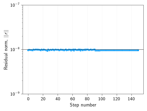
Before, we move on to seeing how the results look like, we need to check if the code is converging to the solution. Fracture is a non-linear problem and to ensure that the reuslts we see are at least numerically correct, we need to check the convergence of the solution. Since we set the tolerance to \(10^{-8}\), we can plot the error per step to see if the solution is converging.
\[
r_\text{norm} = \| \boldsymbol{r} \|
\]
Question
Does the residual norm is always below the tolerance level \(10^{-8}\) for your case for different applied strains? If not, what strategy did you apply to ensure that the solution is converged?
Let us now plot the force-displacement curve. This is the curve that we get by plotting the force on the top surface as a function of the displacement on the top surface. This will tell us how the capacity of the material to carry load changes as the displacement on the top surface increases and the crack propagates.
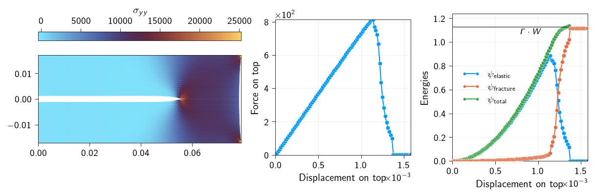
Below we plot the deformed configuration and the force-displacement curve for \(\varepsilon_{applied} = 1.0 \times \varepsilon^0\) at one of the intermediate steps (step number 80). You can run your code for \(\varepsilon_{applied} = 1.0 \times \varepsilon^0\) and check with the plot below to see if your code is correct.
The total energy of the system must be conserved, i.e in order for the crack to propagate, the energy must be dissipated. This energy is taken from the elastic energy of the system. So, if we plot the two energies (elastic and cohesive) as a function of the displacement, we should see that the total energy is conserved. And changes from one to another.
Furthermore, we assumed that the fracture energy (\(\Gamma\)) of the material is constant. Therefore, the total dissipated from crack to propagate through the entire length (\(W\)) of the crack plane would be equal to
\[
\Gamma \cdot{} W
\]
Below, we will plot the elastic and fracture energies as a function of the displacement and loading step to see how the energy is dissipated and changes from one to another.
Question
Comment on what you observe in the force-displacement curve and the energy curves. What is physically happening in the material as the crack propagates?
Code: Plot the deformed configuration, the force-displacement curve and energy curves.
Figure 17.2: Snapshot of deformed configuration with crack propagation at one of the intermediate steps and force-displacement curve, and energy curves. Left: Deformed configuration with stress field in y-direction. Middle: Force-displacement curve. Right: Energy curves.
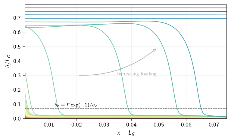
Crack tip opening
Now, let us see how evolution of the crack tip opening along the cohesive line looks like. We compute the jump \([\![\boldsymbol{u}]\!]\) vector at each quadrature point along the cohesive line. We use the line_op operator, defined earlier, to evaluate the jump at the quadrature points of the cohesive line. The quadrature points coordinates are also calculated using the line_op operator.
where \(\boldsymbol{u}_+\) and \(\boldsymbol{u}_-\) are the displacement vectors at the top and bottom of the cohesive line, respectively. Below, we show how to use the eval method of the line_op operator to compute the jump vector at the quadrature points along the cohesive line.
Using this we can compute the opening at the quadrature points along the cohesive line.
Below compute the jump vector at the quadrature points and the opening at the quadrature points along the cohesive line for the last step of the quasistatic problem. Store the opening values in a variable named opening_quadrature.
Now,we do the same for each step of the quasistatic problem. We plot the opening at the quadrature points along the cohesive line for each step. You will have to store the opening values for each step.
Hint
Use the quadrature_points and opening arrays stored at each step to plot the opening along the cohesive line for each step. Remember that the quadrature_points are the coordinates of the quadrature points along the cohesive line and thus the x-coordinates are the same for all the steps.
Figure 17.3: Opening along the cohesive line at different loading steps. The loading steps increase from as the color changes from red to blue. Dashed line indicates the critical opening displacement.
Running the simulation for different applied strains
Now we want to see what happens to this plate configuration when we change the applied strain. We will run the simulation for 3 different applied strains:
So in total, you will run the simulation for 3 different cases. The \(a_c\) is still calculated based on the \(\varepsilon^{0}=1.0\) so the plate geometry doesnot change and the crack length is the same, just the applied strain is changed.
What we want to see is:
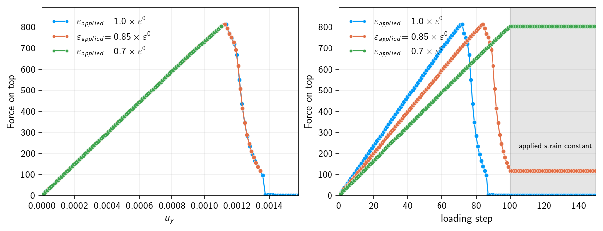
How the force-displacement curve changes with the applied strain?
How the energy distribution (elastic and fracture) changes with the applied strain? Whether for given applied strain, we have enough energy to propagate the crack through the entire length of the cohesive line.
🐍 Download source code
In order to perform the above computations for different applied loadings, we will wrap the code in a function called solve_quasistatic. Click below to download the script that contains the function solve_quasistatic used below.
Import the solve_quasistatic function from the downloaded script. This function is basically all the code that we have written above, wrapped in a function.
Figure 17.4: Load-displacement curves for different applied strains. Left: Load vs displacement curves. Right: Load vs loading step curves.
Energy conservation
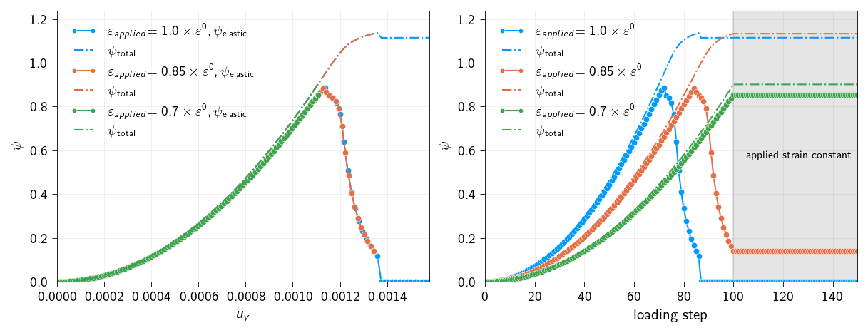
Below, we will plot the elastic and fracture energies as a function of the displacement and loading step to see how the energy is dissipated and changes from one to another.
Question
Plot the elastic energy and the total potential energy curves for
Figure 17.5: Total energy curves (elastic and total energies) for different applied strains. Left: Energy vs displacement curves. Right: Energy vs loading step curves.
as a function of the displacement and loading step.
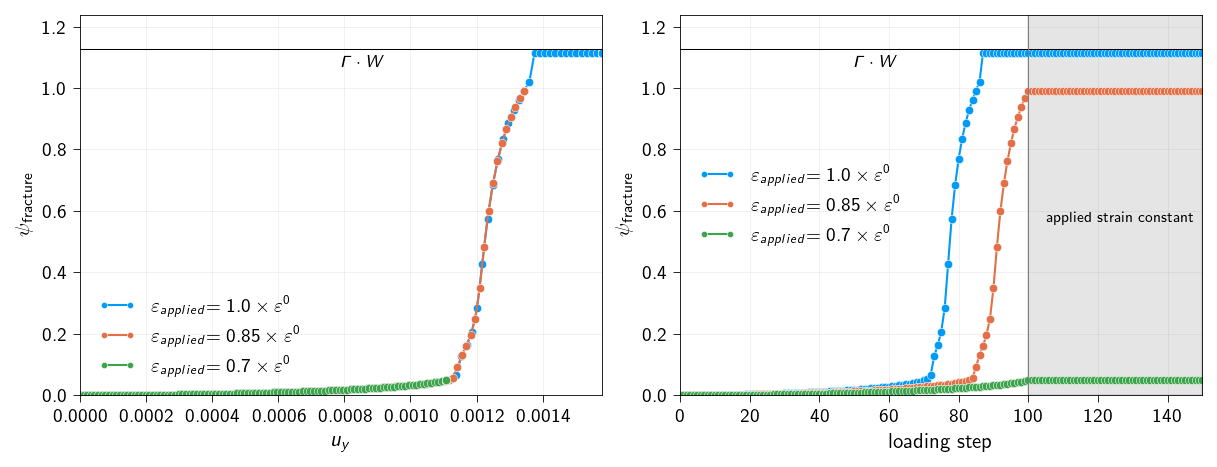
Check if the total dissipated energy is equal to \(\Gamma \cdot{} W\) for all the cases. For which cases, the fracture energy is not equal to \(\Gamma \cdot{} W\)? For the cases where the fracture energy is not equal to \(\Gamma \cdot{} W\), would mean that crack nucleated and only propagated partially. What is the reason for this?
Figure 17.6: Fracture energy curves for different applied strains. Left: Fracture energy vs displacement curves. Right: Fracture energy vs loading step curves.