Matrix-free solvers

In our previous chapter, we efficiently assembled a sparse stiffness matrix. A key step in that process was pre-determining the sparsity pattern—the exact (row, col) locations of all the non-zero entries in the matrix. For a standard and for most of the problems, this pattern is predictable and depends only on the element connectivity.

However, for many advanced and nonlinear problems, the sparsity pattern is not known in advance, or it can even change during the simulation. In that scenario, we cannot use sparse.jacfwd efficiently to build a sparse matrix. Attempting to compute the full, dense Jacobian first and then converting it to a sparse format would be extremely slow and memory-intensive, defeating the purpose of a sparse approach.

This is where matrix-free solvers offer a powerful and elegant solution. They completely bypass the need to know the sparsity pattern because they don’t need to build the matrix at all.

The Core Idea: Action over Existence

Iterative solvers (or Matrix-free solvers) like the Conjugate Gradient (CG) method have a fascinating property: they don’t actually need to “see” the entire matrix \(\mathbf{K}\) at once. All they require is a function that can tell them the action of the matrix on an arbitrary vector \(\boldsymbol{v}\) i.e a function that can compute the matrix-vector product \(\mathbf{K}\boldsymbol{v}\).

This “action” is precisely the Jacobian-Vector Product (JVP). For our system, where the stiffness matrix is the Jacobian of the internal forces, the JVP is:

\[ \mathbf{K}\boldsymbol{v} = \frac{\partial \boldsymbol{f}_{int}}{\partial \boldsymbol{u}} \boldsymbol{v} \]

A matrix-free solver iteratively solves the system \(\mathbf{K}\boldsymbol{u} = \boldsymbol{r}\) by repeatedly calling a JVP function, without ever allocating memory for \(\mathbf{K}\) or needing to know its sparsity pattern. Common methods that can be used in a matrix-free context include:

Conjugate Gradient (CG)
Generalized Minimal Residual (GMRES)
BiConjugate Gradient Stabilized (BiCGSTAB)

The concept of requiring a JVP function goes hand-in-hand with automatic differentiation. As we know from JAX, we can compute the JVP of a function without ever materializing the full Jacobian matrix. This is incredibly powerful because it is:

General: It works for any problem, even when the sparsity pattern is complex, dynamic, or unknown.
Memory Efficient: We avoid storing the massive stiffness matrix

In this chapter, we will see how to construct a JVP function for a stiffness matrix and how to use it to solve a linear system of equations using matrix-free solvers.

How Matrix-Free Methods Work: A Look Inside Conjugate Gradient

As discussed, a matrix-free method solves \(\mathbf{A} \boldsymbol{u} = \boldsymbol{b}\) iteratively using a JVP function instead of the matrix \(\mathbf{A}\) itself. Let’s look at the full algorithm for the Conjugate Gradient (CG) method to see exactly where this happens.

The Conjugate Gradient Algorithm

Given an initial guess \(\boldsymbol{u}_0\), the algorithm proceeds as follows:

Initialization

\(\boldsymbol{r}_0 = \boldsymbol{b} - \mathbf{A} \boldsymbol{u}_0\) (Compute initial residual)
\(\boldsymbol{p}_0 = \boldsymbol{r}_0\) (Set initial search direction)
\(k=0\)

Iteration Loop (Repeat until \(\|\boldsymbol{r}_k\|\) is small enough)

\(\alpha_k = \frac{\boldsymbol{r}_k^T \boldsymbol{r}_k}{\boldsymbol{p}_k^T \mathbf{A} \boldsymbol{p}_k}\) (Compute step size)
\(\boldsymbol{u}_{k+1} = \boldsymbol{u}_k + \alpha_k \boldsymbol{p}_k\) (Update solution)
\(\boldsymbol{r}_{k+1} = \boldsymbol{r}_k - \alpha_k \mathbf{A} \boldsymbol{p}_k\) (Update residual)
\(\beta_k = \frac{\boldsymbol{r}_{k+1}^T \boldsymbol{r}_{k+1}}{\boldsymbol{r}_k^T \boldsymbol{r}_k}\) (Compute improvement factor)
\(\boldsymbol{p}_{k+1} = \boldsymbol{r}_{k+1} + \beta_k \boldsymbol{p}_k\) (Update search direction)
\(k = k+1\)

The Matrix-Free Insight

If you look closely at the algorithm, the matrix \(\mathbf{A}\) is never used for anything other than computing a matrix-vector product. Specifically, it appears only twice inside the loop:

In the denominator for the step size \(\alpha_k\), where we need \(\mathbf{A} \boldsymbol{p}_k\).
In the update for the residual \(\boldsymbol{r}_{k+1}\), where we need \(\mathbf{A} \boldsymbol{p}_k\).

At no point do we need to invert \(\mathbf{A}\), access its individual elements, or know its sparsity pattern. We only need a function that, when given the vector \(\boldsymbol{p}_k\), returns the vector \(\mathbf{A} \boldsymbol{p}_k\).

This is the key to matrix-free methods. We can replace the explicit (and large) stiffness matrix \(\mathbf{A}\) with a much smaller, more efficient JVP function that performs this action. In our JAX-based framework, this is exactly what jax.jvp provides.

Code: Importing libraries

import jax

jax.config.update("jax_enable_x64", True)  # use double-precision
jax.config.update("jax_persistent_cache_min_compile_time_secs", 0)
jax.config.update("jax_platforms", "cpu")
import jax.numpy as jnp
from jax import Array

from jax_autovmap import autovmap

from tatva import Mesh, Operator, element
from tatva.plotting import STYLE_PATH, colors, plot_element_values, plot_nodal_values


from typing import Callable, Optional, Tuple

import numpy as np

import matplotlib.pyplot as plt

Constructing JVP for mechanical problems

Now let us see how we can construct the JVP function for a mechanical problem. We will use the same example of a square domain stretched in the \(x\)-direction.

mesh = Mesh.unit_square(10, 10)

n_nodes = mesh.coords.shape[0]
n_dofs_per_node = 2
n_dofs = n_dofs_per_node * n_nodes

Code: Plotting the mesh

plt.style.use(STYLE_PATH)
plt.figure(figsize=(3, 3), layout="constrained")
plt.tripcolor(
    *mesh.coords.T,
    mesh.elements,
    facecolors=np.ones(mesh.elements.shape[0]),
    edgecolors="k",
    lw=0.2,
    cmap="managua_r",
)
plt.gca().set_aspect("equal")
plt.xlim(0, 1)
plt.ylim(0, 1)
plt.show()

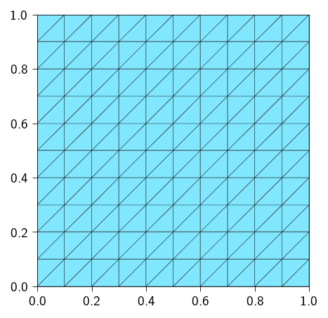
Figure 5.1: Square domain with 10 \(\times\) 10 elements

Defining the total energy

We will assume a linear elastic material and define the strain energy density. Finally, we use the Operator.integrate to integrate the strain energy density over the domain.

\[ \Psi_\text{int}(\boldsymbol{u}) = \int_{\Omega} \frac{1}{2} \boldsymbol{\sigma} : \boldsymbol{\epsilon} ~ d\Omega, \]

where

\[ \boldsymbol{\sigma} = \lambda \text{tr}(\boldsymbol{\epsilon}) \mathbf{I} + 2 \mu \boldsymbol{\epsilon}\qquad\text{and}\qquad\boldsymbol{\epsilon} = \frac{1}{2} (\nabla \boldsymbol{u} + \nabla \boldsymbol{u}^T), \]

The implementation of the above is exactly the same as in all the previous examples. For details, see the code below:

Code: Defining operator and total internal energy

from typing import NamedTuple


class Material(NamedTuple):
    """Material properties for the elasticity operator."""

    mu: float  # Shear modulus
    lmbda: float  # First Lamé parameter


mat = Material(mu=0.5, lmbda=1.0)


@autovmap(grad_u=2)
def compute_strain(grad_u: Array) -> Array:
    """Compute the strain tensor from the gradient of the displacement."""
    return 0.5 * (grad_u + grad_u.T)


@autovmap(eps=2, mu=0, lmbda=0)
def compute_stress(eps: Array, mu: float, lmbda: float) -> Array:
    """Compute the stress tensor from the strain tensor."""
    I = jnp.eye(2)
    return 2 * mu * eps + lmbda * jnp.trace(eps) * I


@autovmap(grad_u=2, mu=0, lmbda=0)
def strain_energy(grad_u: Array, mu: float, lmbda: float) -> Array:
    """Compute the strain energy density."""
    eps = compute_strain(grad_u)
    sig = compute_stress(eps, mu, lmbda)
    return 0.5 * jnp.einsum("ij,ij->", sig, eps)


tri = element.Tri3()
op = Operator(mesh, tri)


@jax.jit
def total_energy(u_flat):
    u = u_flat.reshape(-1, n_dofs_per_node)
    u_grad = op.grad(u)
    energy_density = strain_energy(u_grad, mat.mu, mat.lmbda)
    return op.integrate(energy_density)

JVP function for stiffness matrix

Now let us define the JVP function for the stiffness matrix.We make use of jax.jvp to compute the JVP. The first argument to jax.jvp is the function, the second argument is the input, and the third argument is the perturbation.

\[ \delta \boldsymbol{f}_\text{int} = \frac{\partial \boldsymbol{f}_\text{int}}{\partial \boldsymbol{u}} \delta \boldsymbol{u} \]

The function jax.jvp returns the output of the function which is \(\boldsymbol{f}_\text{int}\) and the Jacobian-Vector product which is the perturbation \(\delta \boldsymbol{f}_\text{int}\). Below we compute the JVP for a small perturbation \(\delta \boldsymbol{u}=0.01\) and compare it with the Jacobian-Vector product computed using jax.jacfwd.

u = jnp.zeros(n_dofs)
delta_u = jnp.full_like(u, fill_value=0.01)

gradient = jax.jacrev(total_energy)
f_jvp, delta_f_jvp = jax.jvp(gradient, (u,), (delta_u,))

In order to check the correctness of the JVP function, we can compute the stiffness matrix using jax.jacfwd and compare the result with the JVP function.

To check if: \(\quad\) jax.jvp(gradient, (u,), (delta_u,))[1] = jax.jacfwd(gradient)(u)@delta_u

K = jax.jacfwd(gradient)(u)
delta_f = K @ delta_u

np.allclose(delta_f, delta_f_jvp, atol=1e-12)

True

How to apply boundary conditions?

The boundary conditions are the same as before. We will apply a displacement of 0.3 to the right boundary. The left boundary is fixed both in the x and y directions.

Code: Finding nodes and dofs to apply boundary conditions

left_nodes = jnp.where(jnp.isclose(mesh.coords[:, 0], 0.0))[0]
right_nodes = jnp.where(jnp.isclose(mesh.coords[:, 0], 1.0))[0]
fixed_dofs = jnp.concatenate(
    [
        2 * left_nodes,
        2 * left_nodes + 1,
        2 * right_nodes,
    ]
)
prescribed_values = jnp.zeros(n_dofs).at[2 * right_nodes].set(0.3)
free_dofs = jnp.setdiff1d(jnp.arange(n_dofs), fixed_dofs)

Applying Dirichlet BCs: The Projection Method

For matrix-free solvers, the correct and exact way to enforce Dirichlet boundary conditions is through projection. This approach, often used in a Projection Conjugate Gradient (PCG) solver, modifies the linear system so that the solution automatically respects the constraints.

The Projection Operator

The core of the method is a projection operator, \(\mathbf{P}\), which we can imagine as a diagonal matrix with: - \(1\) on the diagonal for all free DOFs. - \(0\) on the diagonal for all constrained DOFs.

Applying \(\mathbf{P}\) to any vector zeros out the entries corresponding to the constrained DOFs, effectively projecting it onto the subspace of free DOFs.

The Projected Conjugate Gradient (PCG) Algorithm

Instead of solving \(\mathbf{K}\Delta\boldsymbol{u} = \boldsymbol{r}\), we solve a modified system. The implementation involves these key steps:

Prepare the Right-Hand Side: Compute the full residual vector \(\boldsymbol{r}\). The right-hand side for the solver is then the projected residual:

\[\boldsymbol{b} = \mathbf{P}\boldsymbol{r}\]

Note

The way we do this projection is by setting the \(\boldsymbol{r}\) to zero on the constrained DOFs.

Define the Matrix-Free Operator: The CG solver doesn’t need the matrix, just its action on a vector (the JVP). We define a new JVP function that computes the action of the effective matrix \(\mathbf{K}' = \mathbf{P}\mathbf{K}\mathbf{P}\):

\[ \text{JVP}_{\text{projected}}(\boldsymbol{v}) = \mathbf{P}(\mathbf{K}(\mathbf{P}\boldsymbol{v})) \]

Note

Notice that we project the input vector \(\boldsymbol{v}\) before the JVP and project the output vector after. This ensures that the effective operator is symmetric. The way we do this projection is by setting the \(\boldsymbol{v}\) to zero on the constrained DOFs.

Solve: Run the standard Conjugate Gradient algorithm using the modified right-hand side \(\boldsymbol{b}\) and the new projected JVP function. The initial guess for the solution update should also be in the free subspace (e.g., \(\Delta\boldsymbol{u}_0 = \boldsymbol{0}\)).

The resulting solution \(\Delta\boldsymbol{u}\) is guaranteed to have zeros in all constrained entries.

We start by defining the Jacobian-Vector product. Note that we zero out the constrained DOFs in the vector \(\Delta \boldsymbol{x}\) before computing the JVP and then zero out the constrained DOFs in the output of the JVP. This is the \(\mathbf{P}(\mathbf{K}(\mathbf{P}(\Delta \boldsymbol{x})))\) projection method.

def compute_tangent(dx, x):
    dx_projected = dx.at[fixed_dofs].set(0.0)
    tangent = jax.jvp(gradient, (x,), (dx_projected,))[1]
    tangent = tangent.at[fixed_dofs].set(0)
    return tangent

We define the conjugate gradient solver as a while loop. The first argument is the operator, the second argument is the right-hand-side, the third argument is the tolerance, and the fourth argument is the maximum number of iterations.

def conjugate_gradient_while(A, b, atol=1e-8, max_iter=100):
    iiter = 0

    def body_fun(state):
        b, p, r, rsold, x, iiter = state
        Ap = A(p)
        alpha = rsold / jnp.vdot(p, Ap)
        x = x + jnp.dot(alpha, p)
        r = r - jnp.dot(alpha, Ap)
        rsnew = jnp.vdot(r, r)
        p = r + (rsnew / rsold) * p
        rsold = rsnew
        iiter = iiter + 1
        return (b, p, r, rsold, x, iiter)

    def cond_fun(state):
        b, p, r, rsold, x, iiter = state
        return jnp.logical_and(jnp.sqrt(rsold) > atol, iiter < max_iter)

    x = jnp.full_like(b, fill_value=0.0)
    r = b - A(x)
    p = r
    rsold = jnp.vdot(r, p)

    b, p, r, rsold, x, iiter = jax.lax.while_loop(
        cond_fun, body_fun, (b, p, r, rsold, x, iiter)
    )
    return x, iiter

Now we can define the Newton-Krylov solver using the PCG solver. Notice that we zero out the constrained DOFs in the residual vector. Also, we define the Jacobian-Vector product as a partial function using functools.partial.

from functools import partial


def newton_krylov_solver(
    u,
    fext,
    gradient,
    fixed_dofs,
):
    fint = gradient(u)

    du = jnp.zeros_like(u)

    iiter = 0
    norm_res = 1.0

    tol = 1e-8
    max_iter = 10

    while norm_res > tol and iiter < max_iter:
        residual = fext - fint
        residual = residual.at[fixed_dofs].set(0)
        A = jax.jit(partial(compute_tangent, x=u))
        du, cg_iiter = conjugate_gradient_while(
            A=A, b=residual, atol=1e-8, max_iter=100
        )

        u = u.at[:].add(du)
        fint = gradient(u)
        residual = fext - fint
        residual = residual.at[fixed_dofs].set(0)
        norm_res = jnp.linalg.norm(residual)
        print(f"  Residual: {norm_res:.2e}")
        iiter += 1

    return u, norm_res

Finally we solve the system in 10 steps.

u = jnp.zeros(n_dofs)
fext = jnp.zeros(n_dofs)

n_steps = 10

du_total = prescribed_values / n_steps  # displacement increment
for step in range(n_steps):
    print(f"Step {step + 1}/{n_steps}")
    u = u.at[fixed_dofs].set((step + 1) * du_total[fixed_dofs])

    u_new, rnorm = newton_krylov_solver(
        u,
        fext,
        gradient,
        fixed_dofs,
    )

    u = u_new

u_solution = u.reshape(n_nodes, n_dofs_per_node)

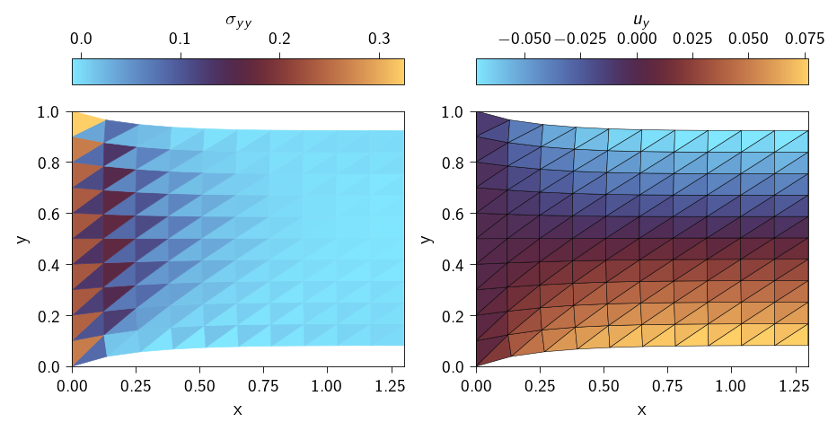
Post-processing

Now we can plot the stress distribution and the displacement.

Code: Plotting the stress distribution

# squeeze to remove the quad point dimension (only 1 quad point)
grad_u = op.grad(u_solution).squeeze()
strains = compute_strain(grad_u)
stresses = compute_stress(strains, mat.mu, mat.lmbda)
plt.style.use(STYLE_PATH)
fig, axs = plt.subplots(1, 2, figsize=(6, 4), layout="constrained")
ax = axs[0]
plot_element_values(
    u=u_solution,
    mesh=mesh,
    values=stresses[:, 1, 1].flatten(),
    ax=ax,
    label=r"$\sigma_{yy}$",
)
ax.set_xlabel(r"x")
ax.set_ylabel(r"y")
ax.set_aspect("equal")
ax.margins(0, 0)

ax = axs[1]
plot_nodal_values(
    u=u_solution,
    mesh=mesh,
    nodal_values=u_solution[:, 1].flatten(),
    ax=ax,
    label=r"$u_y$",
    shading="flat",
    edgecolors="black",
)
ax.set_xlabel(r"x")
ax.set_ylabel(r"y")
ax.set_aspect("equal")

ax.margins(0, 0)
plt.show()

Figure 5.2: Stress distribution after using matrix-free solver