Fundamentals
Multiphysical problems are ubiqutious in engineering and science. Examples include, thermo-mechanical problems, diffusion-driven fracture problems, magneto-elastic problems, etc. In multiphysical problems, the physical processes are coupled and thus the physical quantities (temperature, displacement, etc.) are interdependent. What this means numerically is the solution of one physical process depends on the solution of other physical processes and thus the coupled physical processes need to be solved simultaneously.
A typical energy functional form for a multiphysical problem is given by, \[ \Psi(\mathbf{q}) = \Psi_1(\boldsymbol{q}_1) + \Psi_2(\boldsymbol{q}_2) + \Psi_3(\boldsymbol{q}_3) + \cdots \] where \(\boldsymbol{q} = (\boldsymbol{q}_1, \boldsymbol{q}_2, \boldsymbol{q}_3, \cdots)\) is the field for each physical process and \(\Psi_i\) is the energy functional for the \(i^{th}\) physical process. For example, in a thermo-mechanical problem, \(\boldsymbol{q} = (\boldsymbol{u}, \theta)\) where \(\boldsymbol{u}\) is the displacement field and \(\theta\) is the temperature field. Similarly, in corrosion-driven fracture in concrete, the two physical processes are diffusion of ions and stress buildup from formation of corrosion products. The two fields thus are ionic concentration \(c\) and displacement \(\boldsymbol{u}\).
Thus, our goal is to find the solution \(\boldsymbol{q}\) that minimizes the total energy functional \(\Psi(\boldsymbol{q})\) i.e. \[ \boldsymbol{q} = \arg \min_{\boldsymbol{q}} \Psi(\boldsymbol{q}) \]
In this chapter, we will learn about the fundamentals of multiphysical problems and how to solve them. We will also learn about the different solution strategies to solve coupled problems. For demonstration purpose we will consider the example of a thermo-mechanical problem throughout this chapter. Later in In-class activity: Thermo-mechanical coupling, we will see a practical example of a thermo-mechanical problem involving a bimetallic strip.
The total energy functional for a multiphysical problem can be defined as the sum of the individual energy functionals for each physical process along with a coupling energy functional that describes how the different physical processes interact with each other. For example, in a thermo-mechanical problem, the total energy functional can be written as:
\[ \Psi(u, T) = \Psi_\text{thermal}(T) + \Psi_\text{mechanical}(u) + \Psi_\text{coupling}(u, T) \]
where \(u\) is the displacement field and \(T\) is the temperature field. The thermal energy functional \(\Psi_\text{thermal}(T)\) describes the thermal behavior of the system, the mechanical energy functional \(\Psi_\text{mechanical}(u)\) describes the mechanical behavior of the system, and the coupling energy functional \(\Psi_\text{coupling}(u, T)\) describes how the two process affect each other. Each individual energy functional can be defined as follows: - Thermal energy functional:
\[ \Psi_\text{thermal}(T) = \int_\Omega \left( \frac{1}{2} \kappa |\nabla (T - T_0)|^2 - Q (T - T_0) \right) \, d\Omega \]
where \(\kappa\) is the thermal diffusivity, \(Q\) is the heat source term, and \(\Omega\) is the domain of interest. \(T_0\) is the reference temperature.
- Mechanical energy functional:
\[ \Psi_\text{mechanical}(u) = \int_\Omega \left( \frac{1}{2} \sigma : \varepsilon - f_\text{ext} \cdot u \right) \, d\Omega \]
where \(\sigma\) is the stress tensor, \(\varepsilon\) is the strain tensor, and \(f\) is the body force vector.
- Coupling energy functional:
\[ \Psi_\text{coupling}(u, T) = \int_\Omega -\alpha (3\lambda + 2 \mu) (T - T_0) \, \text{tr}(\varepsilon) \, d\Omega \]
where \(\alpha\) is the thermal expansion coefficient, and \(\lambda\) and \(\mu\) are the Lamé’s parameters.
As mentioned earlier, to find the equilibrium state of the system, we need to minimize the total energy functional \(\Psi(u, T)\) with respect to both the displacement field \(u\) and the temperature field \(T\). This can be done using numerical methods such as the finite element method (FEM). The minimization process involves taking the variation of the total energy functional with respect to both fields and setting it to zero, leading to a coupled set of equations that can be solved simultaneously.
Depending on how the two physical processes are coupled, we can classify multiphysical problems into two categories: one-way coupling and two-way coupling.
One-way coupling (or weak coupling)
When one physical process depends on the solution of another physical process, we say that the two physical processes are coupled. But it does not mean that the two physical processes are coupled in both directions. In one-way coupling, one physical process depends on the solution of another physical process, but the reverse is not true. In the above example of thermo-mechanical coupling, the thermal process cause the expansion/contraction of the body which in turn affects the stress state of the body. However, often it is assumed that the reverse is not true i.e the stress state of the body does not affect the thermal process. This assumption is valid only when the strains are small and the thermal expansion coefficient is small enough such that the effect of mechanical deformation on the thermal process is negligible.
Because of this assumption two physical process are not coupled in both directions, we can solve the two physical processes sequentially i.e. we first solve the thermal process and then use the solution of the thermal process to solve the elasticity problem. The separation of two physical processes give rise to two minimization problem with their own energy functional. This preserves the convexity of the original energy functional and thus even can be solved using a Newton’s method or if the problem is linear, even a linear solver can be used.
This assumption of one-way coupling although simplifies the problem significantly, it may not be valid in all scenarios. In cases where the mechanical deformation significantly affects the thermal process, a two-way coupling approach should be considered. In the rest of the activities we will work with two-way coupling problems as it is more general and more physically accurate.
Two-way coupling (or strong coupling)
When two physical processes are coupled in both directions i.e. the solution of one physical process depends on the solution of the other physical process and vice versa, we say that the two physical processes are coupled in a two-way manner. Therefore, in our thermo-mechanical example, the thermal process affects the mechanical process through thermal expansion/contraction and the mechanical process affects the thermal process through deformation-induced changes in thermal conductivity.
The Fully Coupled (Monolithic) Approach
In the monolithic approach, we treat the entire multiphysics system as a single, unified optimization problem. Rather than distinguishing between mechanical variables (displacement \(\boldsymbol{u}\)) and other physical variables (like temperature \(T\) or phase-field \(\phi\)), we stack every degree of freedom into one massive state vector, \(\mathbf{z}\).
\[ \boldsymbol{z} = \begin{bmatrix} \boldsymbol{u} \\ T \end{bmatrix} \]
To find the equilibrium state, we search for the minimum of the total energy functional \(\Psi_{total}(\mathbf{z})\) by moving in all directions simultaneously. Mathematically, we take the derivative of the energy with respect to the entire vector \(\mathbf{z}\) and set it to zero. This results in a single, giant tangent stiffness matrix (the Hessian) that contains off-diagonal coupling blocks. These blocks, \(\mathbf{K}_{uT}\) and \(\mathbf{K}_{Tu}\), mathematically represent how a change in temperature directly forces a change in displacement, and vice-versa, within a single time step.
\[ \begin{bmatrix} \mathbf{K}_{uu} & \mathbf{K}_{uT} \\ \mathbf{K}_{Tu} & \mathbf{K}_{TT} \end{bmatrix} \begin{Bmatrix} \delta \boldsymbol{u} \\ \delta T \end{Bmatrix} = \begin{Bmatrix} \boldsymbol{R}_u \\ \boldsymbol{R}_T \end{Bmatrix} \]
Physical Insight: The Steepest Descent
You can visualize this approach as a ball rolling down a complex, curved 3D valley. The monolithic solver finds the path of steepest descent by considering the slope and curvature in every direction at once. Physically, this implies that the mechanical and thermal fields equilibrate at the exact same instant. If a small change in temperature causes a massive spike in stress (strong coupling), the solver “sees” this immediately via the coupling blocks and adjusts the solution path to prevent instability. Figure 19.1 illustrates this steepest descent path for a simple coupled energy landscape.
You have actually used a monolithic solver before! Recall how we solved constrained problems using Lagrange multipliers. For example, in Dirichlet BC as constraints (Lagrange multiplier), In-class activity: Active set method and in Assignment 1, where you solved the Herztian contact problem using Lagrange multipliers. We built a KKT system where we stacked the displacements \(\boldsymbol{u}\) and the multipliers \(\boldsymbol{\lambda}\) into a single matrix and solved for them simultaneously. A monolithic multiphysics solver uses the exact same concept, simply replacing the constraint variable \(\lambda\) with a physical variable like temperature.
The key takeaways of the monolithic approach are:
- Simultaneous Physics: All physical fields equilibrate at the exact same instant.
- Robustness: Handles “Strong Coupling” perfectly because the solver sees the interactions (off-diagonal terms) immediately.
- Computationally Heavy: Results in a very large matrix that can be ill-conditioned because it mixes different physical units (e.g., meters and degrees Celsius).
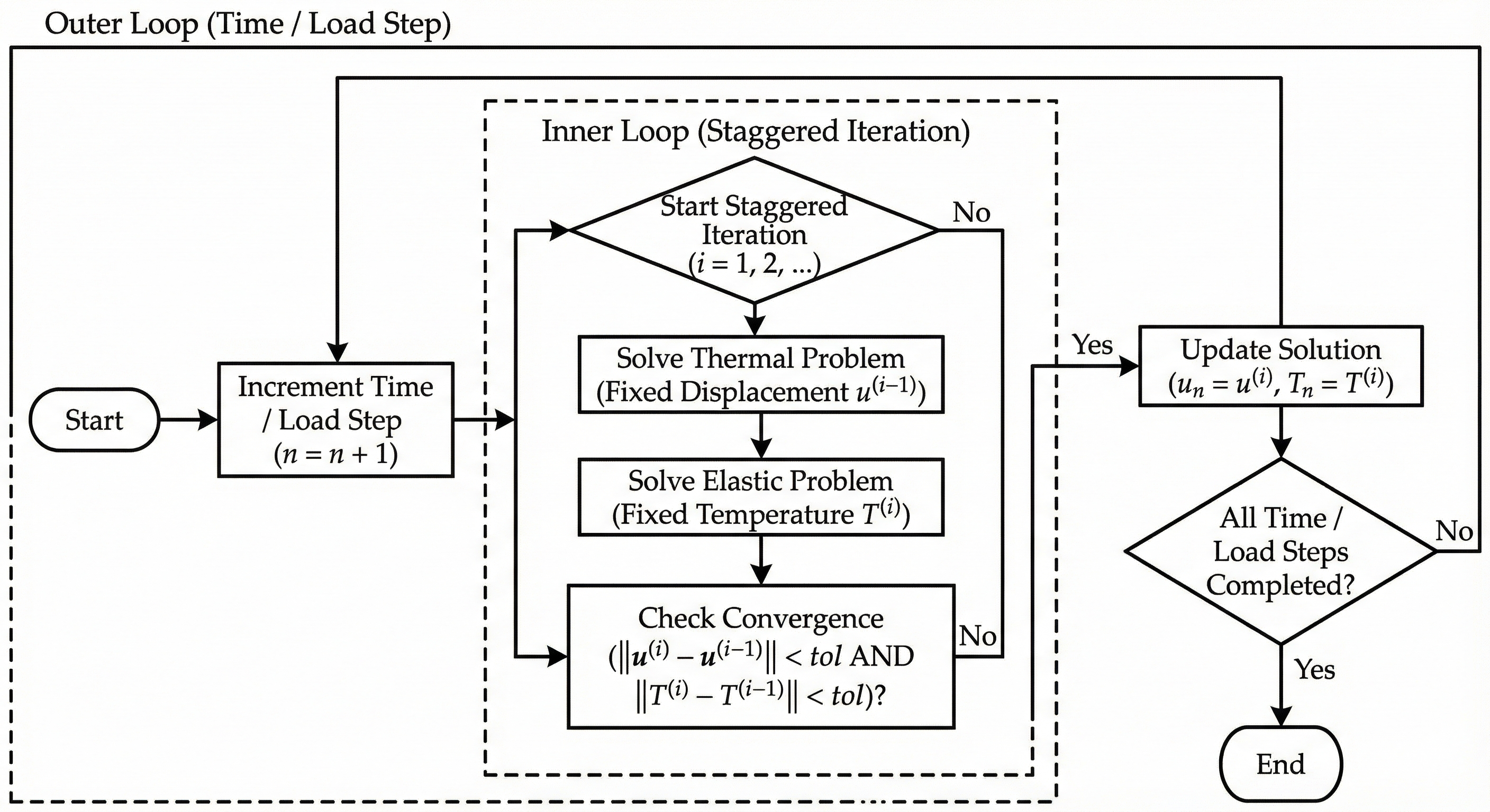
The Staggered (Partitioned) Approach
Often, solving one giant matrix is too computationally expensive or numerically difficult. Instead, we can use a strategy known as Alternate Minimization (or Coordinate Descent). In this approach, we break the complex coupled problem into smaller, manageable pieces.
The algorithm works by “freezing” one physical field while solving for the other. First, we assume the temperature is fixed at its current value (\(T_{old}\)) and minimize the energy with respect to displacement to find \(\boldsymbol{u}_{new}\). Then, we freeze the displacement at this new value and minimize the energy with respect to temperature to find \(T_{new}\). We repeat this “ping-pong” loop until the solution stops changing.
The schematic steps for the staggered approach are shown below:
Physical Insight: The Zig-Zag Path
Returning to our analogy of the valley, the staggered approach is like descending the mountain in a zig-zag pattern. Instead of rolling straight down, you take a step purely in the X-direction, then a step purely in the Y-direction. Physically, this separates the time scales of the physics. It is equivalent to saying: “Let the body deform while keeping the temperature constant (an Isothermal step), and then hold the shape fixed and let the heat diffuse (a Rigid Conduction step).” Figure 19.1 illustrates this zig-zag path for a simple coupled energy landscape.
Why use Staggered if Monolithic is more robust?
While the monolithic approach is theoretically stronger, the staggered approach is often preferred in complex engineering. The total energy landscape of a such complex probelm \(\Psi(\boldsymbol{u}, \phi)\) is often non-convex—picture a wavy surface with many local traps where a solver can get stuck. However, if you slice that landscape along one direction, the partial energies \(\Psi(\boldsymbol{u} | \phi)\) and \(\Psi(\phi | \boldsymbol{u})\) are often convex (simple bowl shapes). It is numerically much easier and more reliable to find the bottom of two simple bowls sequentially than to navigate one complex, wavy surface.
The key takeaways of the staggered approach are:
- Sequential Physics: Processes happen one after the other; one physics “waits” for the other to catch up.
- Modularity: Allows you to use specialized solvers for each physics (e.g., a fast linear solver for heat and a robust Newton solver for mechanics).
- Convexity: In fracture mechanics, splitting the problem often turns one difficult non-convex problem into two solvable convex problems.
- Conditional Stability: Can fail if the coupling is too strong (e.g., if the “zig-zag” steps overshoot the valley floor).
Visual Comparison of Monolithic vs Staggered Solvers
A visual comparison of the two solution strategies is shown below. We can see that the monolithic solver takes a direct path (following the gradient of the energy functional) to the minimum while the staggered solver takes a zig-zag path. For demonstration we chose a very simple coupled energy functional given as
\[ \Psi(u, T) = u^2 + 2T^2 + \frac{1}{4}uT \]