In-class activity: Corrosion-induced stress in concrete
In this activity, we will explore one of the most critical durability issues in civil engineering: corrosion-induced cracking.
When a steel bar embedded in concrete corrodes, it releases iron ions (\(Fe^{2+}\)) that diffuse into the surrounding pore network. These ions react to form rust (iron oxides). The key physical conflict is volume: Rust occupies a much larger volume than the original steel.
This creates a complex, two-way coupled multiphysics problem:
Forward Coupling (Chemistry \(\to\) Mechanics): As rust precipitates, it swells. This exerts massive internal pressure on the concrete, leading to tensile hoop stresses and eventually cracking.
Backward Coupling (Mechanics \(\to\) Chemistry):
Thermodynamic Stifling: As the concrete resists expansion, compressive stress builds up around the pore. This stress acts as an energy barrier, making it thermodynamically unfavorable for more rust to form. Effectively, the pressure increases the solubility limit, stopping the reaction.
Kinetic Clogging: As solid rust fills the pore space, it physically blocks the path, reducing the diffusivity and preventing new ions from entering.
No Coupling
Full Coupling
The Energy Formulation
We model this system using two field variables: the displacement field \(\boldsymbol{u}\) (mechanics) and the molar concentration \(c\) of iron species (chemistry).
We solve this using a Staggered Approach (Alternate Minimization), where we minimize two specific energy functionals sequentially.
Mechanical Energy Functional (Equilibrium)
The concrete seeks to minimize its elastic strain energy. However, the formation of solid rust introduces a Chemical Eigenstrain (\(\boldsymbol{\varepsilon}^*\))—a stress-free expansion that forces the material to deform.
\(\boldsymbol{\varepsilon}\): Total Strain (\(\nabla^s \boldsymbol{u}\)).
\(\mathbb{C}\): Elasticity Tensor (defined by \(E, \nu\)).
\(\boldsymbol{\varepsilon}^*\) (The Coupling): The expansion is zero if the ions are dissolved (\(c < c_{sat}\)). Expansion only occurs for the solid precipitate:
\[
\boldsymbol{\varepsilon}^* = \alpha \cdot \langle c - c_{sat} \rangle_+ \cdot \mathbf{I}
\] where \(\alpha\) is the chemical expansion coefficient and \(\langle \cdot \rangle_+\) is the ramp function.
Chemical Energy Functional (Transport)
The transport of ions is driven by diffusion but resisted by the “clogging” effect. Since diffusion is time-dependent, we minimize an incremental rate potential for each time step \(\Delta t\):
\(\kappa(c)\) (The Clogging): The diffusivity is not constant. It depends on how full the pore is. \[
\kappa(c) = \kappa \cdot \left( 1 - \frac{\text{Amount of Rust}}{\text{Pore Capacity}} \right)
\] As \(c\) increases, \(\kappa(c) \to 0\), shutting down the flow.
The Two-Way Coupling in the Solver
When we minimize the total energy w.r.t. concentration \(c\), the mechanical energy contributes a derivative term: \[
\frac{\partial \Psi_{\text{mech}}}{\partial c} = -3 \sigma_h \Omega
\] This stress term naturally appears in the chemical potential. If the stress \(\sigma_h\) is compressive (negative), this term becomes positive, acting as an energy penalty that stops the diffusion of ions further into the pore and thus halting corrosion.
Workflow
In this activity, we want to observe how each coupling mechanism affects the corrosion-induced cracking process. We will run simulations with different combinations of the coupling effects enabled/disabled.
Case 1: No Coupling (Baseline)
Disable both thermodynamic stifling (\(\alpha = 0\)) and kinetic clogging (\(\kappa(c) = \kappa\))
Observe rapid diffusion of ions and precipitation of rust, but no stress effects.
Case 2: Thermodynamic Stifling Only
Enable the stress-dependent term (\(\alpha > 0\)) but keep constant diffusivity (\(\kappa(c) = \kappa\))
Obeserve buildup of compressive stresses around the pore.
Observe how compressive stresses slow down the corrosion process by comparison to Case 1.
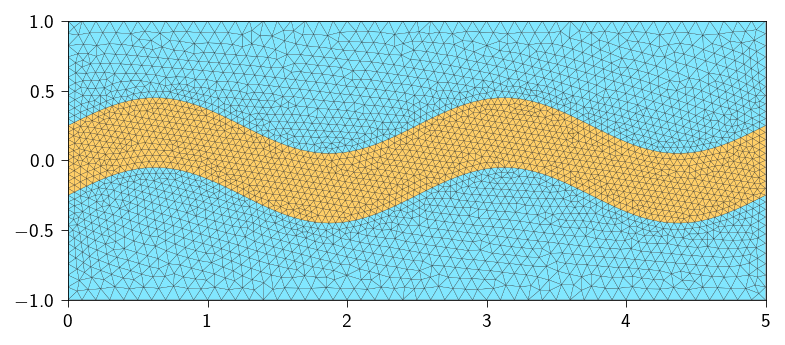
Figure 21.1: Mesh with a wavy pore channel highlighted. Blue: Concrete matrix region with low porosity; Orange: Concrete region with high porosity.
We also need to define two meshes for the concrete matrix region with low porosity and the concrete matrix region with high porosity. We will use these meshes to assign different diffusivity values in the two regions.
matrix_mesh corresponds to the concrete matrix with low porosity,
pore_mesh corresponds to the concrete matrix with high porosity.
Since we will solve the coupled problem using the staggered approach, we need to define the degrees of freedom for each physical problem separately. Lets now define the degrees of freedom for the each physical problem. We will have displacement degrees of freedom for each node in the mesh and concentration degrees of freedom for each node in the mesh.
Since each node has 2 displacement degrees of freedom (for 2D problems) and 1 concentration degree of freedom, the total degrees of each problem will be:
Mechanical problem: \(2 \times \text{number of nodes}\)
Concentration problem: \(1 \times \text{number of nodes}\)
were \(\mu\) and \(\lambda\) are the Lamé’s parameters, \(\boldsymbol{\epsilon}\) is the strain tensor, and \(\mathbf{I}\) is the identity tensor. The elastic strain tensor is defined as:
where \(\kappa(c)\) is the diffusivity parameter that depends on concentration \(c\) of the corrosion species. We define this using a simple relation given as:
where \(\epsilon\) is a small number to avoid numerical issues, \(c_\text{sat}\) is the saturation concentration, and \(\phi_\text{limit}\) is the maximum concentration limit.
Note
Ideally, we should compute the \(\kappa(c)\) based on the current concentration field to accurately capture the effect of clogging on diffusivity. However, this can lead to convergence issues as the problem becomes highly nonlinear. Therefore, we use the concentration from the previous time step \(c_{\text{prev}}\) to compute \(\kappa(c_{\text{prev}})\), which helps in stabilizing the numerical solution. Therefore, we define \(\kappa(c_{\text{prev}})\) as:
where \(c_{\text{prev}}\) is the concentration field from the previous time step at time \(t - \Delta t\).
@jax.jitdef get_clogging_factor(c):""" Calculates diffusivity scaling factor based on precipitate amount. Args: c: Total concentration """# Use jax.nn.relu to handle the "max(0, x)" logic smoothly# RELU is (c - c_sat) if positive, 0 if negative.# precipitate = macaulay_bracket(c - c_sat) precipitate = macaulay_bracket(c - c_sat)#precipitate = jax.nn.relu(c - c_sat)# Calculate the fraction of the pore that is FULL fraction_full = precipitate / pore_capacity# Diffusivity is the remaining empty fraction (1 - full)# We clip it so it never goes below 0.001 (to keep solver stable)# We don't need to clip the top at 1.0 because RELU handles the bottom end,# and fraction_full naturally starts at 0. phi = jnp.clip(1.0- fraction_full, reduction_factor, 1.0)return phi@autovmap(grad_c=1, c=0, c_prev=0, kappa=0)def diffusion_energy_density( grad_c: Array, c: Array, c_prev: Array, kappa: float) -> Array:"""compute diffusion energy density Args: grad_theta (Array): gradient of concentration field c (Array): concentration field at current time step c_prev (Array): concentration field at previous time step kappa (float): diffusivity Returns: Array: diffusion energy density """ kappa_effective = kappa * get_clogging_factor(c_prev)return (0.5* kappa_effective * jnp.einsum("i, i->", grad_c, grad_c)+0.5* ((c - c_prev) **2) / dt )@jax.jitdef total_diffusion_energy(c_flat: Array, c_prev_flat: Array) -> Array:"""Computes the total thermal energy in the bimaterial strip. Args: c_flat (Array): flattened concentration field c_prev_flat (Array): flattened concentration field at previous time step Returns: Array: total diffusion energy """ grad_c_pore = op_pore.grad(c_flat) grad_c_matrix = op_matrix.grad(c_flat) c_pore = op_pore.eval(c_flat) c_matrix = op_matrix.eval(c_flat) c_prev_pore = op_pore.eval(c_prev_flat) c_prev_matrix = op_matrix.eval(c_prev_flat) diffusion_energy_density_matrix = diffusion_energy_density( grad_c_matrix, c=c_matrix, c_prev=c_prev_matrix, kappa=mat_matrix.kappa ) diffusion_energy_density_pore = diffusion_energy_density( grad_c_pore, c=c_pore, c_prev=c_prev_pore, kappa=mat_pore.kappa ) diffusion_energy_matrix = op_matrix.integrate(diffusion_energy_density_matrix) diffusion_energy_pore = op_pore.integrate(diffusion_energy_density_pore)return diffusion_energy_matrix + diffusion_energy_pore
For the concentration problem, we apply a flux boundary condition on the left side (only at the pore inlet) of the strip to simulate the ingress of corrosive species into the pore.
\[
\psi_{\text{c, BC}} = - \int_{\Gamma_q} \bar{q} c \, \text{d}A \quad \text{where} \quad \Gamma_q \text{ is the left edge of the sample, i.e., } x = x_\text{min}~ \text{and}~ y \in \text{pore region}
\]
The corrosive flux \(\bar{q}\) is assumed to be constant over the entire left edge of the sample and is given as
\[
\bar{q} = 1
\]
To compute the corresponding external flux vector, we need to take the variation of this energy term with respect to the concentration field \(c\).
Below we define a few helper functions to compute the external heat flux vector.
Code: Function to extract 1D elements for the top edge of the mesh
def get_elements_on_curve(mesh, curve_func, tol=1e-3): coords = mesh.coords elements_2d = mesh.elements# Efficiently find all nodes on the curve using jax.vmap on_curve_mask = jax.vmap(lambda c: curve_func(c, tol))(coords) elements_1d = []# Iterate through all 2D elements to find edges on the curvefor tri in elements_2d:# Define the three edges of the triangle edges = [(tri[0], tri[1]), (tri[1], tri[2]), (tri[2], tri[0])]for n_a, n_b in edges:# If both nodes of an edge are on the curve, add it to the setif on_curve_mask[n_a] and on_curve_mask[n_b]:# Sort to store canonical representation, e.g., (1, 2) not (2, 1) elements_1d.append(tuple(sorted((n_a, n_b))))ifnot elements_1d:return jnp.array([], dtype=int)return jnp.array(elements_1d)def flux_line(coord: jnp.ndarray, tol: float) ->bool:return jnp.logical_and( jnp.isclose( coord[0], x_min, atol=tol, ), jnp.abs(coord[1]) <= pore_thickness /2, )
We solve the thermo-mechanical problem using a matrix-free Newton-Raphson solver. Now, we define a few functions to implement the matrix-free solvers. We will use the conjugate gradient method to solve the linear system of equations. The Dirichlet boundary conditions are applied using projection method. As we use the matrix-free solver, we need to define the gradient of the total potential energy, which is also the residual function.
Below define the function to compute the \(\boldsymbol{f}_{int}\) using jax.jacrev and then use this function to compute the Jacobian-vector product using jax.jvp. Remember to apply the Projection approach to enforce the Dirichlet boundary conditions.
Remeber we need to define the internal force vector for both diffusion and mechanical problems separately i.e
@eqx.filter_jitdef conjugate_gradient(A, b, atol=1e-8, max_iter=100): iiter =0def body_fun(state): b, p, r, rsold, x, iiter = state Ap = A(p) alpha = rsold / jnp.vdot(p, Ap) x = x + jnp.dot(alpha, p) r = r - jnp.dot(alpha, Ap) rsnew = jnp.vdot(r, r) p = r + (rsnew / rsold) * p rsold = rsnew iiter = iiter +1return (b, p, r, rsold, x, iiter)def cond_fun(state): b, p, r, rsold, x, iiter = statereturn jnp.logical_and(jnp.sqrt(rsold) > atol, iiter < max_iter) x = jnp.full_like(b, fill_value=0.0) r = b - A(x) p = r rsold = jnp.vdot(r, p) b, p, r, rsold, x, iiter = jax.lax.while_loop( cond_fun, body_fun, (b, p, r, rsold, x, iiter) )return x, iiterdef newton_krylov_solver( u, fext, gradient, compute_tangent, fixed_dofs,): fint = gradient(u) iiter =0 norm_res =1.0 tol =1e-8 max_iter =80while norm_res > tol and iiter < max_iter: residual = fext - fint residual = residual.at[fixed_dofs].set(0) A = eqx.Partial( compute_tangent, x_prev=u, gradient=gradient, fixed_dofs=fixed_dofs ) du, cg_iiter = conjugate_gradient(A=A, b=residual, atol=1e-8, max_iter=1000) u = u.at[:].add(du) fint = gradient(u) residual = fext - fint residual = residual.at[fixed_dofs].set(0) norm_res = jnp.linalg.norm(residual) iiter +=1return u, norm_res
Solving the coupled problem
We will use the staggered approach (also known as alternate minimization) to solve the coupled problem. In this approach, we will solve the mechanical and corrosion problems sequentially until convergence is achieved.
Since corrosion is a time-dependent problem, we will solve the coupled problem for each time step. In total we will solve the coupled problem for 500 time steps. The time step size is taken as dt = 0.05.
The time scale for the mechanical problem is much smaller than the time scale for the corrosion problem. Thus, we will assume that the mechanical problem reaches equilibrium instantaneously for each time step of the corrosion problem.
Here are the algorithmic steps corresponding to the code provided. This represents a single-pass operator-split scheme (solving physics sequentially within a time step without iterating to equilibrium between them).
Let \(\boldsymbol{u}_n\) and \(c_n\) be the displacement and concentration fields at time step \(t_n\). Let \(\Delta t\) be the time increment.
1. Time Stepping Loop For each time step \(n = 0, 1, \dots, N\):
2. Diffusion/Corrosion (Transient) Step Solve for the new concentration field \(c_{n+1}\) while holding the mechanical state frozen at the previous configuration \(\boldsymbol{u}_n\).
Find \(c_{n+1}\) such that the first variation of the incremental chemical potential is zero:
\(c_{n+1}\) provides the chemical eigenstrain \(\boldsymbol{\varepsilon}^*(c_{n+1})\) for the constitutive law.
4. Update Store \(\boldsymbol{u}_{n+1}\) and \(c_{n+1}\) and proceed to the next time step.
Hint
The main time-stepping and staggered solution loop is given below. You need to fill in the missing parts to complete the code.
n_steps =2# main load/time stepping loopfor step inrange(n_steps):print(f"Step {step +1}/{n_steps}")# define the external force vectors for diffusion and elastic problem for this step ...# apply the dirichlet boundary conditions for diffusion and elastic problem# also use the previous step concentration field ...# solve for concentration field using the displacement field from previous iteration ...# solve for elastic field using the concentration from above ...
Store the final displacement and concentration fields for ions and the rust for post-processing.
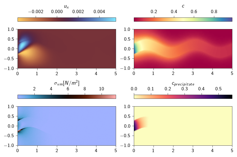
Figure 21.2: Deformed shape of the strip with displacement, von-mises stress, concentration of ferrous ions and precipitation concentration for the full coupling case.
Time evolution of concentration fields
We now plot the time evolution of the concentration field of the ferrous ions and the rust in the concrete specimen over the entire simulation time. We plot the results along the centerline of the specimen (y = 0.).
Code: Function to find the index of the containing polygon for each point.
import numpy as np@jax.jitdef find_containing_polygons( points: jnp.ndarray, polygons: jnp.ndarray,) -> jnp.ndarray:""" Finds the index of the containing polygon for each point. This function uses a vectorized Ray Casting algorithm and is JIT-compiled for maximum performance. It assumes polygons are non-overlapping. Args: points (jnp.ndarray): An array of points to test, shape (num_points, 2). polygons (jnp.ndarray): A 3D array of polygons, where each polygon is a list of vertices. Shape (num_polygons, num_vertices, 2). Returns: jnp.ndarray: An array of shape (num_points,) where each element is the index of the polygon containing the corresponding point. Returns -1 if a point is not in any polygon. """# --- Core function for a single point and a single polygon ---def is_inside(point, vertices): px, py = point# Get all edges of the polygon by pairing vertices with the next one p1s = vertices p2s = jnp.roll(vertices, -1, axis=0) # Get p_{i+1} for each p_i# Conditions for a valid intersection of the horizontal ray from the point# 1. The point's y-coord must be between the edge's y-endpoints y_cond = (p1s[:, 1] <= py) & (p2s[:, 1] > py) | (p2s[:, 1] <= py) & ( p1s[:, 1] > py )# 2. The point's x-coord must be to the left of the edge's x-intersection# Calculate the x-intersection of the ray with the edge x_intersect = (p2s[:, 0] - p1s[:, 0]) * (py - p1s[:, 1]) / ( p2s[:, 1] - p1s[:, 1] ) + p1s[:, 0] x_cond = px < x_intersect# An intersection occurs if both conditions are met. intersections = jnp.sum(y_cond & x_cond)# The point is inside if the number of intersections is odd.return intersections %2==1# --- Vectorize and apply the function ---# Create a boolean matrix: matrix[i, j] is True if point i is in polygon j# Vmap over points (axis 0) and polygons (axis 0)# in_axes=(0, None) -> maps over points, polygon is fixed# in_axes=(None, 0) -> maps over polygons, point is fixed# We vmap the second case over all points is_inside_matrix = jax.vmap(lambda p: jax.vmap(lambda poly: is_inside(p, poly))(polygons) )(points)# Find the index of the first 'True' value for each point (row).# This gives the index of the containing polygon.# We add a 'False' column to handle points outside all polygons.# jnp.argmax will then return the index of this last column. padded_matrix = jnp.pad( is_inside_matrix, ((0, 0), (0, 1)), "constant", constant_values=False ) indices = jnp.argmax(padded_matrix, axis=1)# If the index is the last one, it means the point was not in any polygon.# We map this index to -1 for clarity.return jnp.where(indices == is_inside_matrix.shape[1], -1, indices)
Solid lines represent the concentration of ferrous ions, while dashed lines represent the concentration of rust. Red lines represent the initial time step, while blue lines represent the final time step.
Question
Run the simulation for the four different cases mentioned above and compare the time evolution of the concentration fields (both ferrous ions and rust).
How do the different coupling mechanisms affect the corrosion process? Explain your observations.
To show the effect of each coupling mechanism, plot the concentration profiles for all four cases side by side for comparison.