In-class activity: Thermo-mechanical coupling

In this activity, we will consider an application of two-way coupling. We want to see how one physical process (thermal) affects the other physical process (mechanical) and vice-versa. For the application that we will consider is heating of a bimetallic strip. The strip is made of two different materials, one with a high thermal expansion coefficient and the other with a low thermal expansion coefficient. When the strip is heated, the material with the high thermal expansion coefficient will expand more than the material with the low thermal expansion coefficient. This will cause the strip to bend.

The total energy functional for the coupled thermo-mechanical problem can be written as:

\[ \Psi(u, T) = \Psi_\text{thermal}(T) + \Psi_\text{mechanical}(u) + \Psi_\text{coupling}(u, T) \]

where \(u\) is the displacement field and \(T\) is the temperature field. The thermal energy functional \(\Psi_\text{thermal}(T)\) describes the thermal behavior of the system, the mechanical energy functional \(\Psi_\text{mechanical}(u)\) describes the mechanical behavior of the system, and the coupling energy functional \(\Psi_\text{coupling}(u, T)\) describes how the two process affect each other. Each individual energy functional can be defined as follows:

• Thermal energy functional:

\[ \Psi_\text{thermal}(T) = \int_\Omega \left( \frac{1}{2} \kappa |\nabla (T - T_0)|^2 - Q (T - T_0) \right) \, d\Omega - \int_{\Gamma_q} \bar{q} (T - T_0) \, d\Gamma \]

where \(\kappa\) is the thermal diffusivity, \(Q\) is the heat source term, and \(\Omega\) is the domain of interest. \(T_0\) is the reference temperature. The term on the boundary \(\Gamma_q\) represents the heat flux boundary condition with \(\bar{q}\) being the prescribed heat flux.

• Mechanical energy functional:

\[ \Psi_\text{mechanical}(u) = \int_\Omega \frac{1}{2} \sigma : \varepsilon \, d\Omega - \int_{\Gamma} t_\text{ext} \cdot u \, d\Gamma \]

where \(\sigma\) is the stress tensor, \(\varepsilon\) is the strain tensor, and \(t_\text{ext}\) is the applied traction on the boundary \(\Gamma\).

• Coupling energy functional:

\[ \Psi_\text{coupling}(u, T) = \int_\Omega -\alpha (3\lambda + 2 \mu) (T - T_0) \, \text{tr}(\varepsilon) \, d\Omega \]

where \(\alpha\) is the thermal expansion coefficient, and \(\lambda\) and \(\mu\) are the Lamé’s parameters.

In order to minimize the total energy functional, we need to ensure that the first variation of the total energy functional is zero.

As mentioned in Fundamentals, we can either solve the fully coupled problem using a monolithic approach or use a staggered approach where we solve the thermal and mechanical problems sequentially. As we have seen how to solve a fully coupled problem using a monolithic approach in For example, in Dirichlet BC as constraints (Lagrange multiplier), In-class activity: Active set method and in Assignment 1, we will now focus on the staggered approach.

Staggered approach

In this approach, we assume that the thermal and mechanical problems can be solved sequentially. The conditions for minimization of the total energy functional can be written as:

\[ \dfrac{\partial\Psi}{\partial u} = 0 \quad \text{and} \quad \dfrac{\partial\Psi}{\partial T} = 0 \]

Now,we can solve one problem first and use the solution to solve the other problem. For example, we can first solve the thermal problem to obtain the temperature field \(T\), and then use this temperature field to solve the mechanical problem to obtain the displacement field \(u\).

We will use the finite element method to solve the thermo-mechanical problem and analyze the effect of difference in thermal expansion coefficients on the bending of the strip.

import jax

jax.config.update("jax_enable_x64", True)  # use double-precision
jax.config.update("jax_persistent_cache_min_compile_time_secs", 0)
jax.config.update("jax_platforms", "cpu")
import equinox as eqx
import gmsh
import jax.numpy as jnp
import matplotlib.pyplot as plt
import meshio
from jax import Array
from jax_autovmap import autovmap
from tatva import Mesh, Operator, element
from tatva.plotting import (
    STYLE_PATH,
    colors,
    plot_element_values,
    plot_nodal_values,
)

Model setup

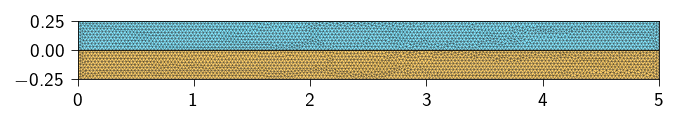
We consider a bimetallic strip of length \(L=5\) m and height \(H=0.5\) m. The strip is made of two materials with different thermal properties.

def generate_bimaterial_mesh(
    width: float,
    height: float,
    mesh_size_far: float,
    mesh_size_interface: float,
    refine_dist_interface: float,
):
    """
    Generates a 2D mesh for two adjacent rectangular blocks with local refinement.

    Args:
        width1 (float): Width of the left block.
        width2 (float): Width of the right block.
        height (float): Common height of the blocks.
        mesh_size_far (float): The general, coarse element size away from refined areas.
        mesh_size_interface (float): The target element size along the common interface.
        refine_dist_interface (float): Distance over which refinement transitions from the interface.
        output_filename (str): Name of the output mesh file.
    """

    import os

    mesh_dir = os.path.join(os.getcwd(), "../meshes")
    os.makedirs(mesh_dir, exist_ok=True)
    output_filename = os.path.join(mesh_dir, "bimaterial_interface.msh")

    gmsh.initialize()
    gmsh.model.add("bimaterial_interface")

    # define the corners of the two blocks and the shared interface.
    p1 = gmsh.model.geo.addPoint(0, -height / 2, 0)
    p2 = gmsh.model.geo.addPoint(width, -height / 2, 0)
    p3 = gmsh.model.geo.addPoint(width, 0, 0)
    p4 = gmsh.model.geo.addPoint(width, height / 2, 0)
    p5 = gmsh.model.geo.addPoint(0, height / 2, 0)
    p6 = gmsh.model.geo.addPoint(0, 0, 0)

    # Define the lines for the boundaries and the interface
    l_bottom = gmsh.model.geo.addLine(p1, p2)
    l_bottom_right = gmsh.model.geo.addLine(p2, p3)
    l_top_right = gmsh.model.geo.addLine(p3, p4)
    l_top = gmsh.model.geo.addLine(p4, p5)
    l_top_left = gmsh.model.geo.addLine(p5, p6)
    l_bottom_left = gmsh.model.geo.addLine(p6, p1)

    # common interface is a single geometric entity shared by both surfaces
    l_interface = gmsh.model.geo.addLine(p6, p3)

    # create the curve loops and surfaces for each block
    loop1 = gmsh.model.geo.addCurveLoop(
        [l_bottom, l_bottom_right, -l_interface, l_bottom_left]
    )
    loop2 = gmsh.model.geo.addCurveLoop([l_interface, l_top_right, l_top, l_top_left])

    surface1 = gmsh.model.geo.addPlaneSurface([loop1])
    surface2 = gmsh.model.geo.addPlaneSurface([loop2])

    # synchronize the model to ensure all entities are recognized
    gmsh.model.geo.synchronize()

    # helps in identifying materials and boundaries when using the mesh file.
    gmsh.model.addPhysicalGroup(2, [surface1], 1, name="bottom")
    gmsh.model.addPhysicalGroup(2, [surface2], 2, name="top")
    gmsh.model.addPhysicalGroup(1, [l_interface], 3, name="interface")

    # refinement along the common interface
    dist_field_interface = gmsh.model.mesh.field.add("Distance", 3)
    gmsh.model.mesh.field.setNumbers(dist_field_interface, "CurvesList", [l_interface])

    thresh_field_interface = gmsh.model.mesh.field.add("Threshold", 4)
    gmsh.model.mesh.field.setNumber(
        thresh_field_interface, "InField", dist_field_interface
    )
    gmsh.model.mesh.field.setNumber(
        thresh_field_interface, "SizeMin", mesh_size_interface
    )
    gmsh.model.mesh.field.setNumber(thresh_field_interface, "SizeMax", mesh_size_far)
    gmsh.model.mesh.field.setNumber(
        thresh_field_interface, "DistMin", refine_dist_interface
    )
    gmsh.model.mesh.field.setNumber(
        thresh_field_interface, "DistMax", refine_dist_interface * 2
    )

    # take the minimum element size prescribed by either refinement rule at any point.
    min_field = gmsh.model.mesh.field.add("Min", 5)
    gmsh.model.mesh.field.setNumbers(min_field, "FieldsList", [thresh_field_interface])

    # set this combined field as the background field to control the mesh generation
    gmsh.model.mesh.field.setAsBackgroundMesh(min_field)

    gmsh.model.mesh.generate(2)
    gmsh.write(output_filename)
    print(f"Mesh successfully generated and saved to '{output_filename}'")

    gmsh.finalize()

    _mesh = meshio.read(output_filename)

    mesh = Mesh(
        coords=_mesh.points[:, :2],
        elements=_mesh.cells_dict["triangle"],
    )

    top_elements_indices = _mesh.cell_sets_dict["top"]["triangle"]
    bottom_elements_indices = _mesh.cell_sets_dict["bottom"]["triangle"]

    interface_elements = _mesh.cells_dict["line"][
        _mesh.cell_sets_dict["interface"]["line"]
    ]

    return mesh, top_elements_indices, bottom_elements_indices, interface_elements

mesh_params = {
    "width": 5.0,
    "height": 0.5,
    "mesh_size_far": 0.03,
    "mesh_size_interface": 0.03,
    "refine_dist_interface": 0.05,
}

mesh, top_elements_indices, bottom_elements_indices, interface_elements = (
    generate_bimaterial_mesh(
        **mesh_params,
    )
)

facecolors = jnp.zeros(mesh.elements.shape[0])
facecolors = facecolors.at[bottom_elements_indices].set(1)

plt.style.use(STYLE_PATH)
plt.figure(figsize=(5, 5))
ax = plt.axes()
ax.tripcolor(
    *mesh.coords.T,
    mesh.elements,
    facecolors=facecolors,
    edgecolors="k",
    lw=0.1,
    cmap="managua_r",
)

ax.axhline(0, color="k", lw=0.4)


ax.set_aspect("equal")
ax.margins(0.0, 0.0)
plt.show()

Mesh with bottom elements colored in green and top elements colored in purple.

We need to also define the two meshes for the top and bottom materials in order to integrate thermal energy density over them separately.

top_mesh = Mesh(mesh.coords, mesh.elements[top_elements_indices])
bottom_mesh = Mesh(mesh.coords, mesh.elements[bottom_elements_indices])

Since we will solve the coupled problem using the staggered approach, we need to define the degrees of freedom for each physical problem separately. Lets now define the degrees of freedom for the each physical problem. We will have displacement degrees of freedom for each node in the mesh and temperature degrees of freedom for each node in the mesh.

Since each node has 2 displacement degrees of freedom (for 2D problems) and 1 temperature degree of freedom, the total degrees of each problem will be:

• Mechanical problem: \(2 \times \text{number of nodes}\)
• Thermal problem: \(1 \times \text{number of nodes}\)

n_nodes = mesh.coords.shape[0]
n_elasticity_dofs_per_node = 2

n_elasticity_dofs = n_elasticity_dofs_per_node * n_nodes
n_thermal_dofs = n_nodes

Material properties

The top part of the strip is made of a material with a thermal diffusivity coefficient of \(\kappa_\text{top}\) and the bottom part is made of a material with a thermal diffusivity coefficient of \(\kappa_\text{bottom}\)., such that

\[ \kappa_\text{top} = 10 \kappa_\text{bottom} \]

where \(\kappa_\text{bottom}=1\) W/m·K.

Similarly, the thermal expansion coefficients of the top \(\alpha_\text{top}\) and bottom materials \(\alpha_\text{bottom}\) are given as:

\[ \alpha_\text{top} = 10 \alpha_\text{bottom} \]

where \(\alpha_\text{bottom}=10^{-5}\) 1/K.

The elastic properties of both materials are assumed to be the same, with a Young’s modulus of \(E=50\) N/m² and a Poisson’s ratio of \(\nu=0.2\).

from typing import NamedTuple


class Material(NamedTuple):
    """Properties of the thermal material"""

    kappa: float  # Thermal diffusivity
    alpha: float  # Thermal expansion coefficient
    mu: float  # Shear modulus
    lmbda: float  # First Lamé parameter


E = 50
nu = 0.2
lmbda = E * nu / (1 + nu) / (1 - 2 * nu)
mu = E / 2 / (1 + nu)


mat_top = Material(kappa=10., alpha=1e-4, mu=mu, lmbda=lmbda)
mat_bottom = Material(kappa=1., alpha=1e-5, mu=mu, lmbda=lmbda)

We now define the Operators for the top and bottom meshes separately to compute the various energy functionals

tri = element.Tri3()
op_top = Operator(top_mesh, tri)
op_bottom = Operator(bottom_mesh, tri)

Defining energy functional for thermal problem

The thermal energy density is given by:

\[ \psi_\text{th} = \frac{1}{2} \kappa (\nabla (T-T_0) \cdot \nabla (T-T_0)) - Q.(T - T_0) \]

where \(\kappa\) is the thermal conductivity, \(Q\) is the heat source per unit volume per unit time, and \(T_0\) is the reference temperature.

Note

For this exercise we assume that reference temperature \(T_0 = 0\) and the heat source \(Q=0\). Therefore, we can simplify the above expressions by removing \(T_0\) and \(Q\).

The thermal functional to be minimized is therefore:

\[ \Psi_\text{th}(T) = \int_{\Omega} \psi_\text{th} \text{d}V - \int_{\Gamma_q} \bar{q} (T - T_0) \, \text{d}A \]

where \(\bar{q}\) is the heat flux on the boundary \(\Gamma_q\).

Since we have two different materials, we need to define the thermal functional for each material.

\[ \Psi_\text{th}(T) = \int_{\Omega_\text{top}} \psi_\text{th} \text{d}V + \int_{\Omega_\text{bottom}} \psi_\text{th} \text{d}V - \int_{\Gamma_q} \bar{q} (T - T_0) \, \text{d}A \]

Hint

For computing the \(\nabla T\) term in the thermal energy density, you can use the op.grad method of the Operator class as we have done in previous activities. Except this time, do not reshape the passed temperature field as it has only 1 degree of freedom, so we can use the flattened temperature field directly.

grad_T = op.grad(T_field.flatten())

@autovmap(grad_theta=1, kappa=0)
def thermal_energy_density(grad_theta: Array, kappa: float) -> Array:
    """compute_thermal energy_density

    Args:
        grad_theta (Array): gradient of temperature field
        kappa (float): thermal conductivity

    Returns:
        Array: thermal energy density
    """

    return 0.5 * kappa * jnp.einsum("i, i->", grad_theta, grad_theta)


@jax.jit
def total_thermal_energy(theta_flat : Array) -> Array:
    """Computes the total thermal energy in the bimaterial strip.
    Args:
        theta_flat (Array): flattened temperature field
    Returns:
        Array: total thermal energy
    """
    
    grad_theta = op_top.grad(theta_flat)
    top_thermal_energy_density = thermal_energy_density(grad_theta, mat_top.kappa)
    top_thermal_energy = op_top.integrate(top_thermal_energy_density)

    grad_theta = op_bottom.grad(theta_flat)
    bottom_thermal_energy_density = thermal_energy_density(grad_theta, mat_bottom.kappa)
    bottom_thermal_energy = op_bottom.integrate(bottom_thermal_energy_density)

    thermal_energy = top_thermal_energy + bottom_thermal_energy
    return thermal_energy

Defining the energy functional for mechanical problem

The total stresses in the strip aare given as

\[ \boldsymbol{\sigma} = 2 \mu \boldsymbol{\epsilon} + \lambda \text{tr}(\boldsymbol{\epsilon}) \mathbf{I} \]

were \(\mu\) and \(\lambda\) are the Lamé’s parameters, \(\boldsymbol{\epsilon}\) is the strain tensor, and \(\mathbf{I}\) is the identity tensor. The strain tensor is defined as:

\[ \boldsymbol{\epsilon} = \frac{1}{2} \left( \nabla \mathbf{u} + (\nabla \mathbf{u})^T \right) \]

The total elastic energy is thus given by:

\[ \Psi_\text{elastic} = \int_{\Omega} \frac{1}{2} \boldsymbol{\sigma} : \boldsymbol{\epsilon} ~\text{d}\Omega \]

where \(\Omega\) is the domain of the strip.

Since the elastic properties are the same for both materials, we can define a single operator for the elastic problem.

@autovmap(grad_u=2)
def compute_strain(grad_u: Array) -> Array:
    """Compute the strain tensor from the gradient of the displacement."""
    return 0.5 * (grad_u + grad_u.T)


@autovmap(eps=2, mu=0, lmbda=0)
def compute_stress(eps: Array, mu: float, lmbda: float) -> Array:
    """Compute the stress tensor from the strain tensor."""
    I = jnp.eye(2)
    return 2 * mu * eps + lmbda * jnp.trace(eps) * I


@autovmap(grad_u=2, mu=0, lmbda=0)
def strain_energy_density(grad_u: Array, mu: float, lmbda: float) -> Array:
    """Compute the strain energy density.
    
    Args:
        grad_u (Array): Gradient of the displacement field.
        mu (float): Shear modulus.
        lmbda (float): First Lamé parameter.
    Returns:
        Array: Strain energy density.
    """
    eps = compute_strain(grad_u)
    sig = compute_stress(eps, mu, lmbda)
    return 0.5 * jnp.einsum("ij,ij->", sig, eps)


@jax.jit
def total_elastic_energy(u_flat: Array) -> Array:
    """Computes the total elastic energy in the bimaterial strip.
    Args:
        u_flat (Array): flattened displacement field
    Returns:
        Array: total elastic energy
    """
    
    u = u_flat.reshape(-1, n_elasticity_dofs_per_node)
    u_grad_top = op_top.grad(u)
    u_grad_bottom = op_bottom.grad(u)

    elasticity_energy_density_bottom = strain_energy_density(
        u_grad_bottom, mu=mat_bottom.mu, lmbda=mat_bottom.lmbda
    )

    elasticity_energy_density_top = strain_energy_density(
        u_grad_top, mu=mat_top.mu, lmbda=mat_top.lmbda
    )

    elastic_energy_top = op_top.integrate(elasticity_energy_density_top)
    elastic_energy_bottom = op_bottom.integrate(elasticity_energy_density_bottom)

    return elastic_energy_top + elastic_energy_bottom

Define coupling energy functional

The coupling energy functional describes how the thermal process affects the mechanical process. The coupling energy density is given by:

\[ \psi_\text{coupling} = -\alpha (3\lambda + 2 \mu) (T - T_0) \, \text{tr}(\varepsilon) \]

and results in the following coupling energy functional:

\[ \Psi_\text{coupling}(u, T) = \int_\Omega \psi_\text{coupling} \, d\Omega \]

@autovmap(grad_u=2, theta_quad=0, mu=0, lmbda=0, alpha=0)
def coupling_energy_density(
    grad_u: Array, theta_quad: Array, mu: float, lmbda: float, alpha: float
) -> Array:
    """Compute the coupling energy density between thermal and elastic fields.
    
    Args:
        grad_u (Array): Gradient of the displacement field.
        theta_quad (Array): Temperature at quadrature points.
        mu (float): Shear modulus.
        lmbda (float): First Lamé parameter.
        alpha (float): Thermal expansion coefficient.
    Returns:
        Array: Coupling energy density.
    """

    eps = compute_strain(grad_u)
    I = jnp.eye(2)
    return -alpha * (3 * lmbda + 2 * mu) * theta_quad * jnp.trace(eps)


@jax.jit
def total_coupling_energy(u_flat: Array, theta_flat: Array) -> Array:
    """Computes the total coupling energy in the bimaterial strip.
    Args:
        u_flat (Array): flattened displacement field
        theta_flat (Array): flattened temperature field
    Returns:
        Array: total coupling energy
    """
    
    u = u_flat.reshape(-1, n_elasticity_dofs_per_node)
    u_grad_top = op_top.grad(u)
    u_grad_bottom = op_bottom.grad(u)

    theta_quad_top = op_top.eval(theta_flat)
    theta_quad_bottom = op_bottom.eval(theta_flat)

    coupling_energy_density_top = coupling_energy_density(
        u_grad_top,
        theta_quad_top,
        mu=mat_top.mu,
        lmbda=mat_top.lmbda,
        alpha=mat_top.alpha,
    )
    coupling_energy_density_bottom = coupling_energy_density(
        u_grad_bottom,
        theta_quad_bottom,
        mu=mat_bottom.mu,
        lmbda=mat_bottom.lmbda,
        alpha=mat_bottom.alpha,
    )

    coupling_energy_top = op_top.integrate(coupling_energy_density_top)
    coupling_energy_bottom = op_bottom.integrate(coupling_energy_density_bottom)

    return coupling_energy_top + coupling_energy_bottom

Define the total energy functional

\[ \Psi_\text{total}(u, T) = \Psi_\text{el}(u) + \Psi_\text{coup}(u, T) + \Psi_\text{th}(T) \]

Note

If you notice the units of thermal properties have Watts (W) which is Joules per second (J/s). Therefore, the thermal energy functional actually represents a rate of energy (power). To be consistent with the mechanical energy functional which has units of energy (Joules), we need to multiply the thermal energy functional by a time step \(\Delta t\) (in seconds) to convert it to energy. For simplicity, we can assume \(\Delta t = 1\) s.

@jax.jit
def total_energy(u_flat: Array, theta_flat: Array) -> Array:
    elastic_energy = total_elastic_energy(u_flat)
    coupling_energy = total_coupling_energy(u_flat, theta_flat)
    thermal_energy = total_thermal_energy(theta_flat)
    return elastic_energy + coupling_energy + thermal_energy

def total_energy_elastic(u_flat: Array, theta_flat: Array) -> Array:
    return total_energy(u_flat=u_flat, theta_flat=theta_flat)

def total_energy_thermal(theta_flat: Array, u_flat: Array, ) -> Array:
    return total_energy(u_flat=u_flat, theta_flat=theta_flat)

Defining boundary conditions for thermal problem

Since the thermal process is independent of the elastic process, we can solve the thermal problem first.

The Dirichlet boundary condition is applied on the left, right and bottom sides of the strip. We maintain the temperature at these boundaries to be \(0^\circ\) C. \[ T(x=x_\text{min}) = 0^\circ \text{C}, \quad T(x=x_\text{max}) = 0^\circ \text{C}, \quad T(y=y_\text{min}) = 0^\circ \text{C} \]

x_max = mesh.coords[:, 0].max()
x_min = mesh.coords[:, 0].min()
y_max = mesh.coords[:, 1].max()
y_min = mesh.coords[:, 1].min()

left_nodes = jnp.where(jnp.isclose(mesh.coords[:, 0], x_min))[0]
right_nodes = jnp.where(jnp.isclose(mesh.coords[:, 0], x_max))[0]
top_nodes = jnp.where(jnp.isclose(mesh.coords[:, 1], y_max))[0]
bottom_nodes = jnp.where(jnp.isclose(mesh.coords[:, 1], y_min))[0]
fixed_dofs_th = jnp.concatenate(
    [
        right_nodes,
        left_nodes,
        bottom_nodes,
    ]
)
prescribed_values_th = jnp.zeros(n_thermal_dofs)
prescribed_values_th = prescribed_values_th.at[right_nodes].set(0.0)
prescribed_values_th = prescribed_values_th.at[left_nodes].set(0.0)
prescribed_values_th = prescribed_values_th.at[bottom_nodes].set(0.0)

free_dofs_th = jnp.setdiff1d(jnp.arange(n_thermal_dofs), fixed_dofs_th)

We define a Neumann boundary condition (heat flux \(\bar{q}\)) on the top edge of the strip. As mentioned earlier, the energy associatd with this boundary condition is given by:

\[ \psi_{\text{th, BC}} = - \int_{\Gamma_q} \bar{q} T \, \text{d}A \quad \text{where} \quad \Gamma_q \text{ is the top edge of the strip, i.e., } y = y_\text{max} \]

The heat flux \(\bar{q}\) is assumed to be constant over the entire top edge of the strip and is given as

\[ \bar{q} = 20~ \text{W/m²} \]

To compute the corresponding external heat flux vector, we need to take the variation of this energy term with respect to the temperature field \(T\).

\[ \boldsymbol{f}_\text{ext, th} = - \dfrac{\partial \psi_{\text{th, BC}}}{\partial T} \]

Below we define a few helper functions to compute the external heat flux vector.

def get_elements_on_curve(mesh, curve_func, tol=1e-3):
    coords = mesh.coords
    elements_2d = mesh.elements
    # Efficiently find all nodes on the curve using jax.vmap
    on_curve_mask = jax.vmap(lambda c: curve_func(c, tol))(coords)

    elements_1d = []
    # Iterate through all 2D elements to find edges on the curve
    for tri in elements_2d:
        # Define the three edges of the triangle
        edges = [(tri[0], tri[1]), (tri[1], tri[2]), (tri[2], tri[0])]
        for n_a, n_b in edges:
            # If both nodes of an edge are on the curve, add it to the set
            if on_curve_mask[n_a] and on_curve_mask[n_b]:
                # Sort to store canonical representation, e.g., (1, 2) not (2, 1)
                elements_1d.append(tuple(sorted((n_a, n_b))))

    if not elements_1d:
        return jnp.array([], dtype=int)

    return jnp.array(elements_1d)


def heat_flux_line(coord: jnp.ndarray, tol: float) -> bool:
    return jnp.isclose(
        coord[1],
        y_max,
        atol=tol,
    )

heat_flux_elements = get_elements_on_curve(mesh, heat_flux_line, tol=1e-8)

line_mesh = Mesh(mesh.coords, heat_flux_elements)
line2 = element.Line2()
line_op = Operator(line_mesh, line2)


@jax.jit
def flux_energy(x_flat: Array, q_bar: float) -> Array:
    u_quad = op_top.eval(x_flat).flatten()
    return line_op.integrate(q_bar * u_quad)

q_bar = 20.0 # External heat flux magnitude

fext_th = jax.jacrev(flux_energy)(jnp.ones(n_nodes), q_bar)

Defining boundary conditions for mechanical problem

We fix the displacement of the strip on the left edges in both \(x\) and \(y\) directions.

\[ u_x(x=x_\text{min}) = 0, \quad u_y(x=x_\text{min}) = 0 \]

We assume no external forces are applied to the strip i.e \(f_\text{ext, elas}=0\)

fixed_dofs_u = jnp.concatenate(
    [
        2 * left_nodes,
        2 * left_nodes + 1,
    ]
)
prescribed_values_u = jnp.zeros(n_elasticity_dofs)
free_dofs_u = jnp.setdiff1d(jnp.arange(n_elasticity_dofs), fixed_dofs_u)

Using Matrix-Free solver

We solve the thermo-mechanical problem using a matrix-free Newton-Raphson solver. Now, we define a few functions to implement the matrix-free solvers. We will use the conjugate gradient method to solve the linear system of equations. The Dirichlet boundary conditions are applied using projection method. As we use the matrix-free solver, we need to define the gradient of the total potential energy, which is also the residual function.

\[ \boldsymbol{r} = \frac{\partial \Psi}{\partial \boldsymbol{u}} = \boldsymbol{f}_{int} - \boldsymbol{f}_{ext} \]

We also define a function to compute the JVP product to compute the incremental residual for an increment in the displacement.

\[ \delta \boldsymbol{r} = \frac{\partial \boldsymbol{r}}{\partial \boldsymbol{u}}|_{\boldsymbol{u}=\boldsymbol{u}_\mathrm{prev}} \delta \boldsymbol{u} \]

Hint

Below define the function to compute the \(\boldsymbol{f}_{int}\) using jax.jacrev and then use this function to compute the Jacobian-vector product using jax.jvp. Remember to apply the Projection approach to enforce the Dirichlet boundary conditions.

Remeber we need to define the internal force vector for both thermal and mechanical problems separately i.e

\[ \boldsymbol{f}_\text{int, th} = \dfrac{\partial \Psi_\text{total}(T, \boldsymbol{u})}{\partial T} \]

\[ \boldsymbol{f}_\text{int, elas} = \dfrac{\partial \Psi_\text{total}(\boldsymbol{u}, T)}{\partial \boldsymbol{u}} \]

Similarly, we need to define the JVP functions for both thermal and mechanical problems separately.

gradient_elastic = jax.jacrev(total_energy_elastic, argnums=0)
gradient_thermal = jax.jacrev(total_energy_thermal, argnums=0)

@eqx.filter_jit
def compute_tangent(dx, x_prev, gradient, fixed_dofs):
    dx_projected = dx.at[fixed_dofs].set(0)
    tangent = jax.jvp(gradient, (x_prev,), (dx_projected,))[1]
    tangent = tangent.at[fixed_dofs].set(0)
    return tangent

Below we define the Conjugate-gradient method and the Newton-Rahpson method to solve the nonlinear problem of contact. See Matrix-free solvers, In-class activity: Node-to-Surface Contact and In-class activity: Cohesive zone modelling for more details on how to implement Conjugate-gradient and Newton-Raphson methods for matrix-free solvers.

@eqx.filter_jit
def conjugate_gradient(A, b, atol=1e-8, max_iter=100):
    iiter = 0

    def body_fun(state):
        b, p, r, rsold, x, iiter = state
        Ap = A(p)
        alpha = rsold / jnp.vdot(p, Ap)
        x = x + jnp.dot(alpha, p)
        r = r - jnp.dot(alpha, Ap)
        rsnew = jnp.vdot(r, r)
        p = r + (rsnew / rsold) * p
        rsold = rsnew
        iiter = iiter + 1
        return (b, p, r, rsold, x, iiter)

    def cond_fun(state):
        b, p, r, rsold, x, iiter = state
        return jnp.logical_and(jnp.sqrt(rsold) > atol, iiter < max_iter)

    x = jnp.full_like(b, fill_value=0.0)
    r = b - A(x)
    p = r
    rsold = jnp.vdot(r, p)

    b, p, r, rsold, x, iiter = jax.lax.while_loop(
        cond_fun, body_fun, (b, p, r, rsold, x, iiter)
    )
    return x, iiter


def newton_krylov_solver(
    u,
    fext,
    gradient,
    compute_tangent,
    fixed_dofs,
):
    fint = gradient(u)

    iiter = 0
    norm_res = 1.0

    tol = 1e-8
    max_iter = 80
 
    while norm_res > tol and iiter < max_iter:
        residual = fext - fint
        residual = residual.at[fixed_dofs].set(0)
        A = eqx.Partial(
            compute_tangent, x_prev=u, gradient=gradient, fixed_dofs=fixed_dofs
        )
        du, cg_iiter = conjugate_gradient(A=A, b=residual, atol=1e-8, max_iter=1000)

        u = u.at[:].add(du)
        fint = gradient(u)
        residual = fext - fint
        residual = residual.at[fixed_dofs].set(0)
        norm_res = jnp.linalg.norm(residual)
        iiter += 1

    return u, norm_res

Solving thermo-mechanical problem

Now, we will solve the thermo-mechanical problem using the staggered approach. In order to solve, we first solve the thermal problem to obtain the temperature field, and then use this temperature field to solve the mechanical problem to obtain the displacement field.

We will apply the external heat flux \(\boldsymbol{f}_\text{ext, th}\) in 2 steps n_steps=2. In each step, we will perform staggered iterations (max 5) to solve the thermal and mechanical problems sequentially until convergence. Within each staggered iteration, we will first solve the thermal problem using the displacement field from the previous iteration, and then solve the mechanical problem using the temperature field from the previous iteration. We will check for convergence by computing the relative change in displacement and temperature fields given as

\[ \| \boldsymbol{u}^{i} - \boldsymbol{u}^{i-1}\|, ~ \text{and} ~ \| T^{i} - T^{i-1} \| \]

If the relative change is less than a tolerance of 1e-8, we will stop the staggered iterations for that step i.e we have converged to a solution.

Hint

The main time-stepping and staggered solution loop is given below. You need to fill in the missing parts to complete the code.

n_steps = 2

# main load/time stepping loop
for step in range(n_steps):
    print(f"Step {step + 1}/{n_steps}")

    # define the external force vectors for thermal and elastic problem for this step
    ...

    # apply the dirichlet boundary conditions for thermal and elastic problem
    ...


    # the staggered solution loop, we perform 5 staggered iterations
    for i in range(5):

        print(f"===Staggered iteration {i + 1}/5:===")
        
        # solve for thermal field using the displacement field from previous iteration
        ...
        
        # solve for elastic field using the temperature field from previous iteration
        ...

        # compute the relative change in displacement and temperature fields
        err_u = ...
        err_T = ...
        
        # check if err_u and err_T are less than tolerance (1e-8), if yes then break the staggered loop
        ...

Store the final displacement and temperature fields for post-processing.

u_solution = ...
T_solution = ...

n_steps = 2

u = jnp.zeros(n_elasticity_dofs)
theta = jnp.zeros(n_thermal_dofs)

fext_u = jnp.zeros(n_elasticity_dofs)

fext_theta = jnp.zeros(n_thermal_dofs)

dtheta_total = prescribed_values_th / n_steps  # displacement increment
du_total = prescribed_values_u / n_steps  # temperature increment

dfxt_th = fext_th / n_steps

u_per_step = []
theta_per_step = []

for step in range(n_steps):
    print(f"Step {step + 1}/{n_steps}")
    u = u.at[fixed_dofs_u].add(du_total[fixed_dofs_u])
    theta = theta.at[fixed_dofs_th].add(dtheta_total[fixed_dofs_th])

    fext_theta = fext_theta.at[:].add(dfxt_th)

    for i in range(5):
        u_prev = u
        theta_prev = theta

        print(f"===Staggered iteration {i + 1}/5:===")
        # solve for thermal field
        print(" Solving for thermal field")
        partial_gradient_thermal = eqx.Partial(
            gradient_thermal, u_flat=u_prev.flatten()
        )

        theta, rnorm = newton_krylov_solver(
            theta_prev,
            fext=fext_theta,
            gradient=partial_gradient_thermal,
            compute_tangent=compute_tangent,
            fixed_dofs=fixed_dofs_th,
        )
        print(f"    Residual norm in thermal solve: {rnorm:.8e}")

        # solve for elastic field
        print(" Solving for elastic field")

        partial_gradient_elastic = eqx.Partial(
            gradient_elastic, theta_flat=theta.flatten()
        )

        u, rnorm = newton_krylov_solver(
            u=u_prev,
            fext=fext_u,
            gradient=partial_gradient_elastic,
            fixed_dofs=fixed_dofs_u,
            compute_tangent=compute_tangent,
        )
        print(f"    Residual norm in elastic solve: {rnorm:.8e}")

        err_u = jnp.linalg.norm(u - u_prev) #/ jnp.linalg.norm(u_prev + 1e-16)
        err_theta = jnp.linalg.norm(theta - theta_prev) #/ jnp.linalg.norm(theta_prev + 1e-16)

        print(f"  Relative change in u: {err_u:.8e}, theta: {err_theta:.8e}")

        if err_u < 1e-8 and err_theta < 1e-8:
            print(f"  Converged in {i + 1} staggered iterations.")
            break

    u_per_step.append(u_prev.reshape(n_nodes, n_elasticity_dofs_per_node))
    theta_per_step.append(theta_prev.reshape(n_nodes,))

u_solution = u.reshape(n_nodes, n_elasticity_dofs_per_node)
T_solution = theta.reshape(
    n_nodes,
)

Step 1/2
===Staggered iteration 1/5:===
 Solving for thermal field
    Residual norm in thermal solve: 9.39190850e-09
 Solving for elastic field
    Residual norm in elastic solve: 9.79290835e-09
  Relative change in u: 1.79070725e-01, theta: 9.10442094e+01
===Staggered iteration 2/5:===
 Solving for thermal field
    Residual norm in thermal solve: 9.26784913e-09
 Solving for elastic field
    Residual norm in elastic solve: 9.81493143e-09
  Relative change in u: 0.00000000e+00, theta: 8.84185501e-06
===Staggered iteration 3/5:===
 Solving for thermal field
    Residual norm in thermal solve: 9.26784913e-09
 Solving for elastic field
    Residual norm in elastic solve: 9.81493143e-09
  Relative change in u: 0.00000000e+00, theta: 0.00000000e+00
  Converged in 3 staggered iterations.
Step 2/2
===Staggered iteration 1/5:===
 Solving for thermal field
    Residual norm in thermal solve: 9.37487337e-09
 Solving for elastic field
    Residual norm in elastic solve: 9.70249768e-09
  Relative change in u: 1.79070742e-01, theta: 9.10442094e+01
===Staggered iteration 2/5:===
 Solving for thermal field
    Residual norm in thermal solve: 9.88887850e-09
 Solving for elastic field
    Residual norm in elastic solve: 9.73265785e-09
  Relative change in u: 0.00000000e+00, theta: 8.84174138e-06
===Staggered iteration 3/5:===
 Solving for thermal field
    Residual norm in thermal solve: 9.88887850e-09
 Solving for elastic field
    Residual norm in elastic solve: 9.73265785e-09
  Relative change in u: 0.00000000e+00, theta: 0.00000000e+00
  Converged in 3 staggered iterations.

Note

You will notice that in each staggered iteration, individual problems converge (the rnorm for each problem is below tolerance) but the overall staggered step doesnot converge i.e. the errors in displacements and temperatures do not reduce significantly:

\[ \| \boldsymbol{u}^{i} - \boldsymbol{u}^{i-1}\| > 10^{-8}, ~ \text{and} ~ \| T^{i} - T^{i-1} \| > 10^{-8} \]

where \(i\) is the staggered iteration number.

This is because for each problem we assumed that the other problem is fixed. However, in reality both problems are coupled and affect each other. Furthermore, we chose to solve the thermal problem first and then the mechanical problem. This also introduces some error in the combined solution.

Therefore, we need to perform multiple staggered iterations to ensure that both problems converge to a consistent solution.

Plot the deformed shape of the strip

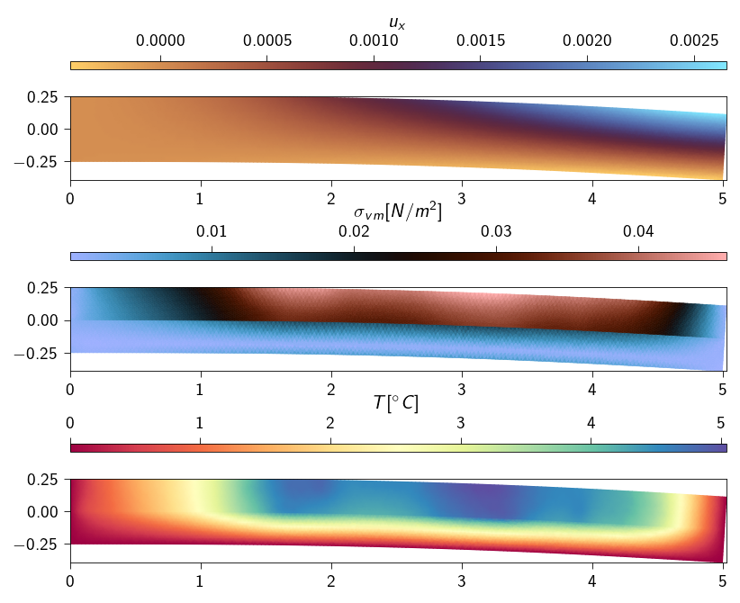
We now plot the deformed shape of the strip along with displacement, von Mises stress and temperature values. We can observe that the strip has bended with top surface expanding more than the bottom part.

@autovmap(stress=2)
def von_mises_stress(stress):
    s_xx, s_yy = stress[0, 0], stress[1, 1]
    s_xy = stress[0, 1]
    return jnp.sqrt(s_xx**2 - s_xx * s_yy + s_yy**2 + 3 * s_xy**2)

plt.style.use(STYLE_PATH)
fig, axs = plt.subplots(
    3, 1, figsize=(8, 4), layout="constrained", gridspec_kw={"hspace": 0.25}
)

plot_nodal_values(
    mesh=mesh,
    nodal_values=u_solution[:, 0],
    u=u_solution,
    ax=axs[0],
    cmap="managua",
    scale=10.0,
    label=r"$u_x$",
)
axs[0].set_aspect("equal")
axs[0].margins(0.0, 0.0)

op = Operator(mesh, tri)


grad_u = op.grad(u_solution).squeeze()
strains = compute_strain(grad_u)
theta_quad = op.eval(T_solution).squeeze()
stresses = compute_stress(strains, mat_top.mu, mat_top.lmbda)
stress_vm = von_mises_stress(stresses)

plot_element_values(
    mesh=mesh,
    values=stress_vm.flatten(),
    u=u_solution,
    ax=axs[1],
    cmap="berlin",
    scale=10.0,
    label=r"$\sigma_{vm} [N/m^2]$",
)
axs[1].set_aspect("equal")
axs[1].margins(0.0, 0.0)

plot_nodal_values(
    mesh=mesh,
    nodal_values=T_solution,
    u=u_solution,
    ax=axs[2],
    cmap="Spectral",
    scale=10.0,
    label=r"$T [^\circ C]$",
)
axs[2].set_aspect("equal")
axs[2].margins(0.0, 0.0)

plt.show()

Deformed shape of the strip with displacement, von-misesstress and temperature fields. Deformation have been magnified by 10 times for better visibility.

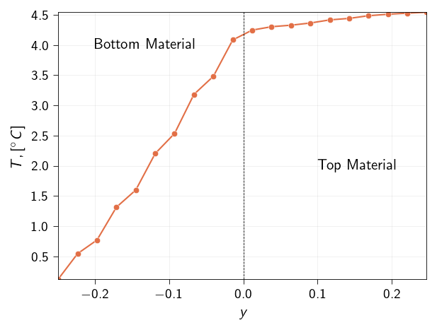
We can also plot the temperature field on the both side of the strip. We define a operator to evaluate the temperature at quadrature points, find the indices of the elements that contains the points where we want to evaluate the temperature and then interpolate the temperature at the points.

import numpy as np


@jax.jit
def find_containing_polygons(
    points: jnp.ndarray,
    polygons: jnp.ndarray,
) -> jnp.ndarray:
    """
    Finds the index of the containing polygon for each point.

    This function uses a vectorized Ray Casting algorithm and is JIT-compiled
    for maximum performance. It assumes polygons are non-overlapping.

    Args:
        points (jnp.ndarray): An array of points to test, shape (num_points, 2).
        polygons (jnp.ndarray): A 3D array of polygons, where each polygon is a
                                list of vertices. Shape (num_polygons, num_vertices, 2).

    Returns:
        jnp.ndarray: An array of shape (num_points,) where each element is the
                     index of the polygon containing the corresponding point.
                     Returns -1 if a point is not in any polygon.
    """

    # --- Core function for a single point and a single polygon ---
    def is_inside(point, vertices):
        px, py = point

        # Get all edges of the polygon by pairing vertices with the next one
        p1s = vertices
        p2s = jnp.roll(vertices, -1, axis=0)  # Get p_{i+1} for each p_i

        # Conditions for a valid intersection of the horizontal ray from the point
        # 1. The point's y-coord must be between the edge's y-endpoints
        y_cond = (p1s[:, 1] <= py) & (p2s[:, 1] > py) | (p2s[:, 1] <= py) & (
            p1s[:, 1] > py
        )

        # 2. The point's x-coord must be to the left of the edge's x-intersection
        # Calculate the x-intersection of the ray with the edge
        x_intersect = (p2s[:, 0] - p1s[:, 0]) * (py - p1s[:, 1]) / (
            p2s[:, 1] - p1s[:, 1]
        ) + p1s[:, 0]
        x_cond = px < x_intersect

        # An intersection occurs if both conditions are met.
        intersections = jnp.sum(y_cond & x_cond)

        # The point is inside if the number of intersections is odd.
        return intersections % 2 == 1

    # --- Vectorize and apply the function ---
    # Create a boolean matrix: matrix[i, j] is True if point i is in polygon j
    # Vmap over points (axis 0) and polygons (axis 0)
    # in_axes=(0, None) -> maps over points, polygon is fixed
    # in_axes=(None, 0) -> maps over polygons, point is fixed
    # We vmap the second case over all points
    is_inside_matrix = jax.vmap(
        lambda p: jax.vmap(lambda poly: is_inside(p, poly))(polygons)
    )(points)

    # Find the index of the first 'True' value for each point (row).
    # This gives the index of the containing polygon.
    # We add a 'False' column to handle points outside all polygons.
    # jnp.argmax will then return the index of this last column.
    padded_matrix = jnp.pad(
        is_inside_matrix, ((0, 0), (0, 1)), "constant", constant_values=False
    )
    indices = jnp.argmax(padded_matrix, axis=1)

    # If the index is the last one, it means the point was not in any polygon.
    # We map this index to -1 for clarity.
    return jnp.where(indices == is_inside_matrix.shape[1], -1, indices)

op = Operator(mesh, tri)
T_quad = op.eval(T_solution).squeeze()

y = np.linspace(y_min, 0.99*y_max, 20)
x = np.full_like(y, fill_value=x_max / 2)

points = np.stack([x, y], axis=1)
mid_containing_indices = find_containing_polygons(points, mesh.coords[mesh.elements])

plt.style.use(STYLE_PATH)
plt.figure(figsize=(4, 3), layout="constrained")
ax = plt.axes()

ax.plot(
    y,
    T_quad[mid_containing_indices],
    "o-",
    color=colors.red,
)
ax.axvline(x=0, color="k", lw=0.4, ls="--")
ax.text(-0.2, 4, "Bottom Material", va="center")
ax.text(0.1, 2, "Top Material", va="center")
ax.set_xlabel(r"$y$")
ax.set_ylabel(r"$T, [^\circ C]$")
ax.grid(True)
ax.margins(0.0, 0.0)
plt.show()

Figure 20.1: Temperature field on the strip